Five worked examples
Five models solved with OGR Slip2D 0.1.235. For each one we give the figure computed by the program, the data needed to check it and the .ogr file, so you can open it yourself. All the numbers on this page come from the program.
A two-layer slope with a water table
A 16 m high cut with a bench, in silty sand over clay on a base of dense gravel, with a water table crossing the slope. It is the same model that the quick start builds step by step. The automatic grid places 169 centres above the slope and tries 11 radii at each, 1 859 circles in all.
- Silty sand
- c′ = 5 kPa · φ′ = 32° · γ = 19 kN/m³
- Clay
- c′ = 12 kPa · φ′ = 24° · γ = 19.5 kN/m³
- Dense gravel
- c′ = 0 · φ′ = 40° · γ = 21 kN/m³
- Search
- Grid 12 × 12, 11 radii per centre, 30 slices
| Method | F |
|---|---|
| Bishop simplified | 1.300 |
| Spencer (λ = 0.343) | 1.290 |
| GLE / Morgenstern–Price | 1.292 |
An embankment on soft clay with a weak seam
A 6 m embankment on soft clay whose undrained strength grows with depth, with a thin weak seam 4.5 m below the ground. The critical surface is non-circular and runs along the seam. A berm at the toe is the usual remedy, and comparing the two models shows how much it raises the factor of safety.
- Fill
- c′ = 5 kPa · φ′ = 32° · γ = 20 kN/m³ · slope 2H:1V
- Soft clay
- su = 18 kPa at the ground, + 1.5 kPa/m with depth · γ = 16.5 kN/m³
- Weak seam
- su = 12 kPa · γ = 16 kN/m³ · at y = −4.5 m
- Firm clay
- su = 60 kPa · γ = 19 kN/m³ · below y = −8 m
| Model | Search | Spencer | GLE |
|---|---|---|---|
| 2a · no berm | Block, polyline along the seam | 0.988 | 0.990 |
| 2a · no berm | Path, 5 000 surfaces | 0.978 | 0.985 |
| 2b · berm | Block, polyline along the seam | 1.180 | 1.168 |
Both searches find the same mechanism; Figure 3.4.5 shows the one found by the path search. The analysis is in total stresses, without pore pressure.
An earth dam: steady seepage and stability
A homogeneous dam 15 m high, with the reservoir at 13 m and a toe drain 16 m long. The finite-element seepage analysis gives the free surface and the pore pressure at the base of each slice, and the drain keeps the water away from the downstream face.
- Section
- Crest 6 m · upstream 3H:1V · downstream 2.5H:1V · on an impervious base
- Fill
- c′ = 8 kPa · φ′ = 30° · γ = 20 kN/m³
- Hydraulics
- Ks = 10⁻⁶ m/s, isotropic · van Genuchten α = 3.6 m⁻¹, n = 1.56
- Conditions
- H = 13 m on the upstream face · P = 0 on the drain · seepage face elsewhere · no flow through the base
| Result | Value |
|---|---|
| Pore pressure in the dam | up to 127.5 kPa |
| Seepage-face nodes | 0 |
| Downstream slope, Bishop simplified | 1.800 |
| Downstream slope, Spencer (λ = 0.322) | 1.799 |
The mesh and the head field are shown in Figure 3.7.1, and the pore pressure on the slices of the critical surface in Figure 3.7.5.
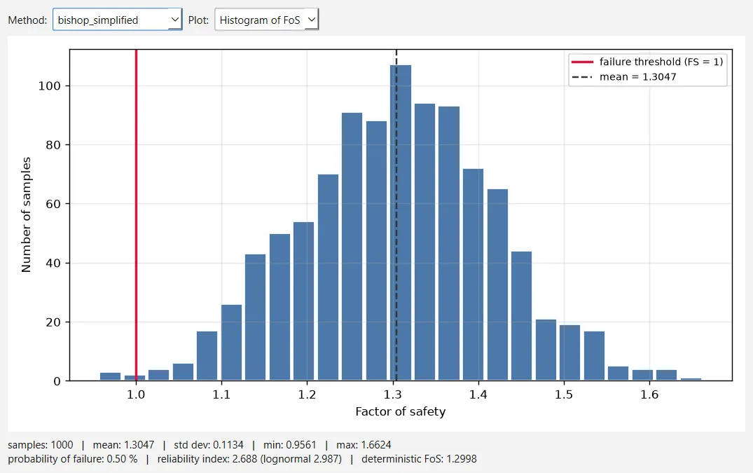
The slope of example 1 with uncertain strengths
Three strength parameters become random variables, each normal and truncated at three standard deviations. We evaluate 1 000 Monte Carlo samples on the deterministic critical surface of each method (global minimum).
- Clay c′
- mean 12 kPa · σ = 3 kPa · 3 to 21 kPa
- Clay φ′
- mean 24° · σ = 2.4° · 16.8° to 31.2°
- Silty sand φ′
- mean 32° · σ = 2° · 26° to 38°
| Method | Mean F | σF | PF | β | βln |
|---|---|---|---|---|---|
| Bishop simplified | 1.305 | 0.113 | 0.5 % | 2.69 | 2.99 |
| Spencer | 1.295 | 0.114 | 0.5 % | 2.60 | 2.88 |
| GLE / Morgenstern–Price | 1.298 | 0.113 | 0.5 % | 2.63 | 2.91 |
Only five of the 1 000 samples fall below 1, which is too few to pin the probability down, as the convergence plot shows.
Rapid drawdown as a transient seepage problem
This is the dam of example 3, but here we look at its upstream slope while the reservoir is lowered from 13 m to 1 m in eight days. The finite-element analysis follows the water as it drains out of the fill, and a full search finds the factor of safety at the end of each stage. The lowest factor of safety comes two days after the reservoir reaches its lowest level.
| Day | Reservoir | F (Spencer) |
|---|---|---|
| 0 | 13.0 m · steady | 2.604 |
| 2 | 10.6 m | 2.193 |
| 4 | 8.2 m | 1.851 |
| 6 | 5.8 m | 1.651 |
| 8 | 3.4 m | 1.519 |
| 10 | 1.0 m | 1.469 |
| 20 | 1.0 m | 1.526 |
| 50 | 1.0 m | 1.641 |
Seven stages with 20 time steps each. A stage applies its level from the end of the previous stage, so the level drops by 2.4 m on days 0, 2, 4, 6 and 8, and each factor of safety is computed at the end of its stage. The stages at 10 and 20 days report time steps that did not reach the tolerance of 10−5; with the automatic number of steps instead, each of the factors above changed by less than 0.002. The same curve appears as Figure 3.8.4 in the theory manual.
How to reproduce the examples
Each file opens in OGR Slip2D 0.1.235 with the settings used on this page: press Compute and compare the result with the tables. An AI agent connected through the MCP server can also open the files and explain the results.