OGR Slip2D
A desktop program for two-dimensional slope stability by limit equilibrium, with a finite-element groundwater engine, probabilistic analysis and an official MCP server. The source code is public, so you can read every equation the program uses.
Why we developed OGR Slip2D
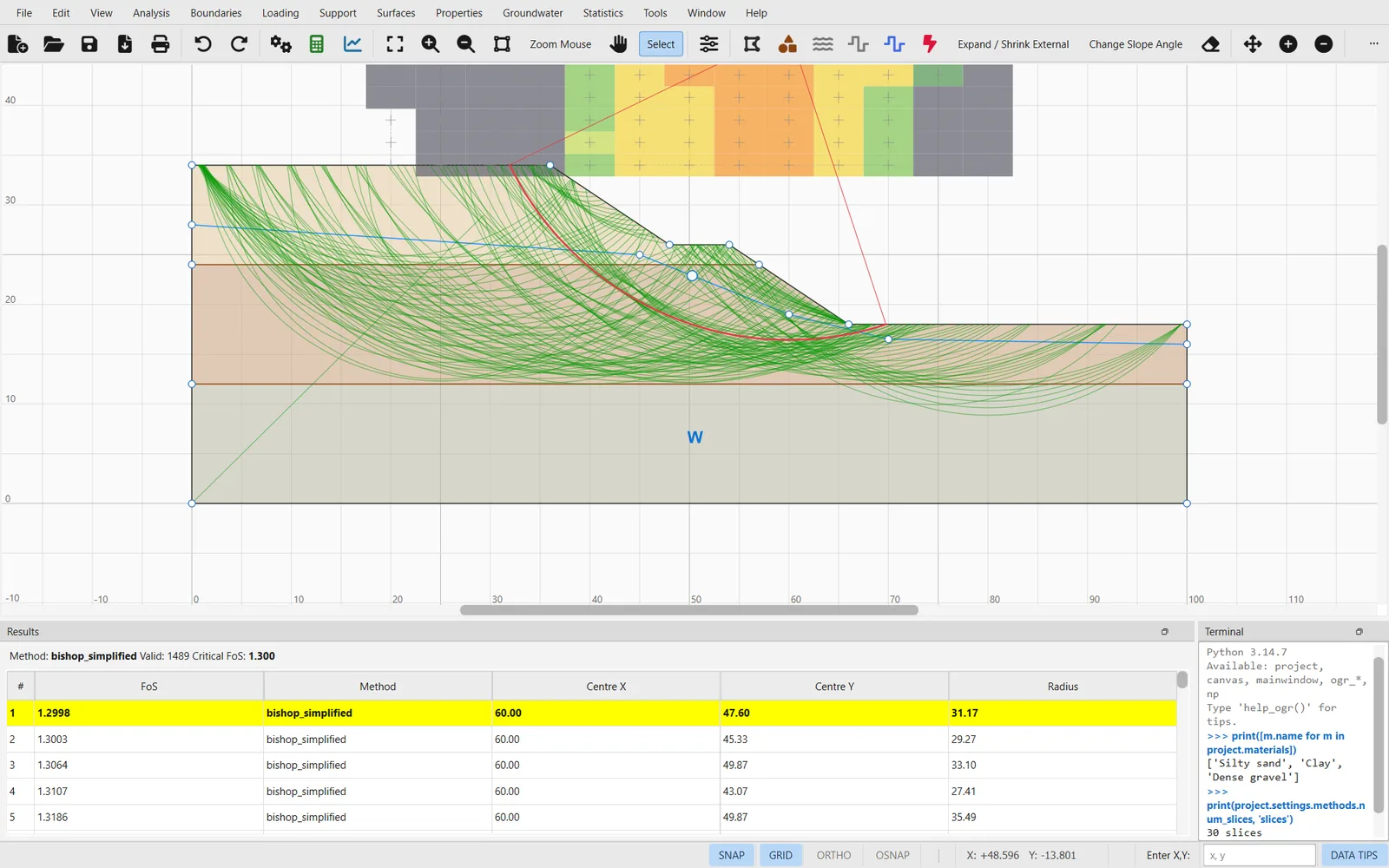
Most of the software geotechnical engineers rely on is closed: if a factor of safety comes out at 1.32, there is no way to see how the program got there. OGR Slip2D is a new implementation, in plain Python, of the analysis practitioners run most often. It has a graphical interface and a test suite that anyone can inspect, and each method comes with the reference case it was validated against.
Nine methods and seven search algorithms
You can run several methods in one analysis and compare their critical surfaces. The program handles circular, non-circular and composite surfaces, weak layers, slope limits and optimisation of the critical surface, and its focus objects filter the search before any surface is evaluated.
Each method has been validated against a published case or the slice tables of a reference manual. From the simplest to the most rigorous:
| Method | Equilibrium |
|---|---|
| Ordinary / Fellenius | moment |
| Bishop simplified | moment |
| Janbu simplified · corrected | force |
| Corps of Engineers #1 · #2 | force |
| Lowe–Karafiath | force |
| Spencer | force + moment |
| GLE / Morgenstern–Price | force + moment |
Circular: grid, slope, auto-refine and particle swarm. Non-circular: block (with window, line, point and polyline objects), path, simulated annealing, auto-refine and particle swarm.
Focus objects (a window, a line, a point or a tangent) discard candidate surfaces before they are evaluated. In the reference case, a tangent to a weak layer cuts the evaluations from 206 to 17. Non-circular critical surfaces can be optimised by a random walk.
How each search works →Twenty-two strength models, each with its parameters in the units of the project:
Mohr–Coulomb · undrained · undrained varying with depth, datum or distance to the slope · drained–undrained · SHANSEP · vertical stress ratio
Hoek–Brown · generalised Hoek–Brown with a GSI calculator · Barton–Bandis · power curve · hyperbolic
Anisotropic linear · modified anisotropic linear · anisotropic strength function · generalised anisotropic
Shear–normal function · discrete function · c/φ function · infinite strength · no strength (water)
Seepage computed by finite elements
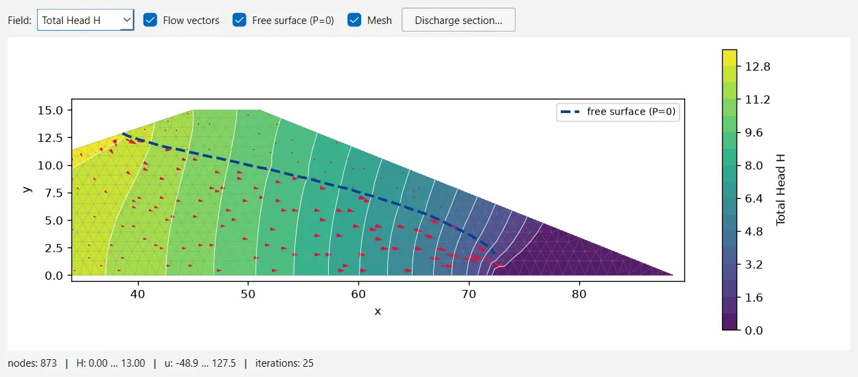
- Triangular meshes over the material regions, with shared nodes along the interfaces between materials.
- Saturated steady flow with an anisotropic conductivity tensor for each material.
- Unsaturated flow with six permeability functions: simple, Brooks–Corey, Fredlund–Xing, Gardner, van Genuchten and user-defined.
- The phreatic surface and the seepage faces are found by switching the boundary condition node by node.
- Transient analysis in stages, with the mixed form of Richards' equation and a factor of safety for each stage. In a rapid drawdown, this gives the factor of safety as a function of time.
- When no seepage analysis is needed: water tables, piezometric lines, ru, pressure grids, ponded water and B̄ excess pore pressure.
Probability of failure and sensitivity analysis
- Random variables for strengths, unit weights, hydraulic properties, supports, loads, seismic coefficients and the water table.
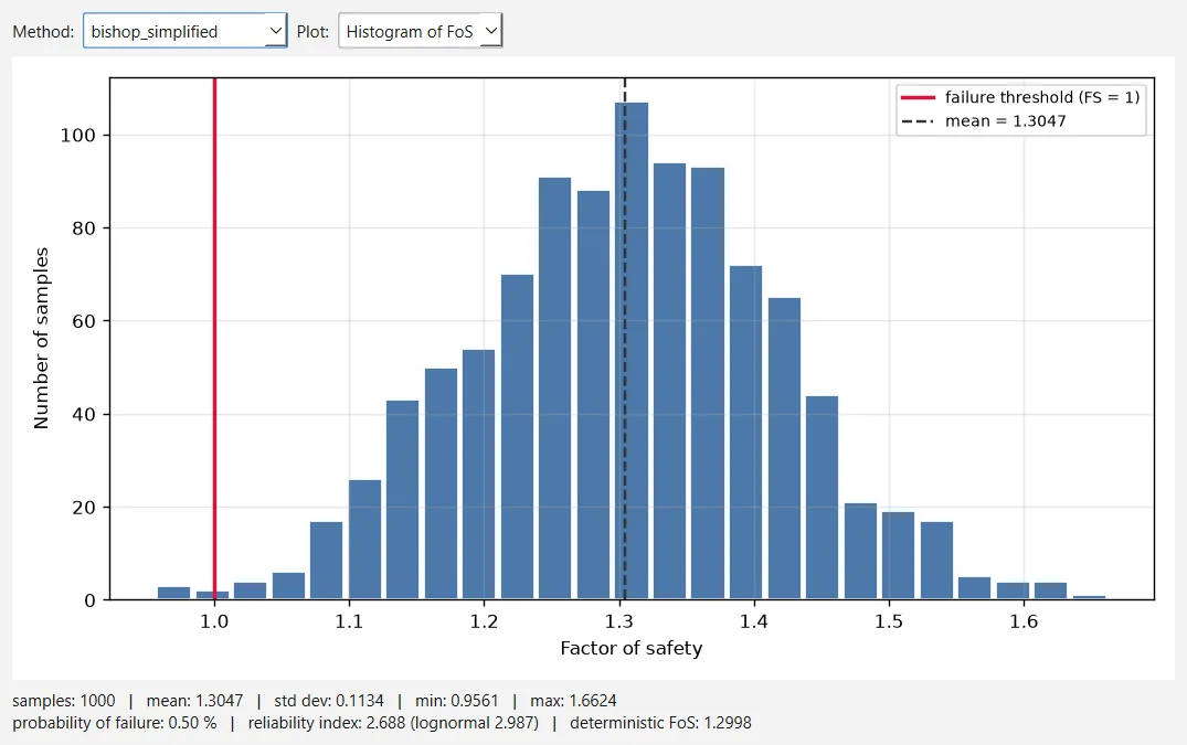
- Seven distributions with relative truncation, Monte Carlo or Latin hypercube sampling, and correlation between cohesion and friction.
- Global-minimum and overall-slope analyses, probability of failure, reliability index, convergence plots and the critical probabilistic surface.
- Sensitivity sweeps that rank the inputs by their influence on the factor of safety.
Loads, supports and design codes
A section can carry supports, external loads and seismic action, and the design checks can follow Eurocode 7. The program also reads and writes DXF drawings, produces reports and can be driven by scripts.
Supports
End-anchored, grouted tieback (with and without friction), soil nail, pile or micropile, geosynthetic, helical anchor, retaining wall by equivalent fluid pressure, and user-defined. Supports can be active or passive, and a back analysis finds the force needed for a target factor of safety.
Loads and seismic
Distributed and line loads with five orientations, pseudo-static seismic coefficients and tension cracks with water. The program also finds the yield acceleration and, from acceleration records, the Newmark sliding-block displacement.
Eurocode 7
Partial factors for design approaches DA1-C1, DA1-C2, DA2 and DA3, or factors of your own. They are applied to a copy of the model, so the calculation does not modify your project.
DXF import and export
DXF import with layer detection and geometry clean-up, and DXF export of the model and the critical surfaces. Annotations, dimensions and images can be added on the canvas.
Reports
PDF reports of an analysis, property tables, images of the canvas in bitmap or SVG, and CSV exports of surfaces and slices.
Scripting
An embedded Python terminal with access to the open model, a command-line interface for batch runs, a Python API and the MCP server for AI agents.
The three steps of an analysis
They are the same in the desktop program, from Python or through an agent. The model is a plain JSON .ogr file that all three can open.
Draw or import
Boundaries are drawn with the mouse, typed in as coordinates or imported from DXF. Then you assign materials to regions and add water, loads and supports.
Search and solve
Each enabled method runs its search in the background, in parallel where possible, with a progress bar and a cancel button.
Read the result
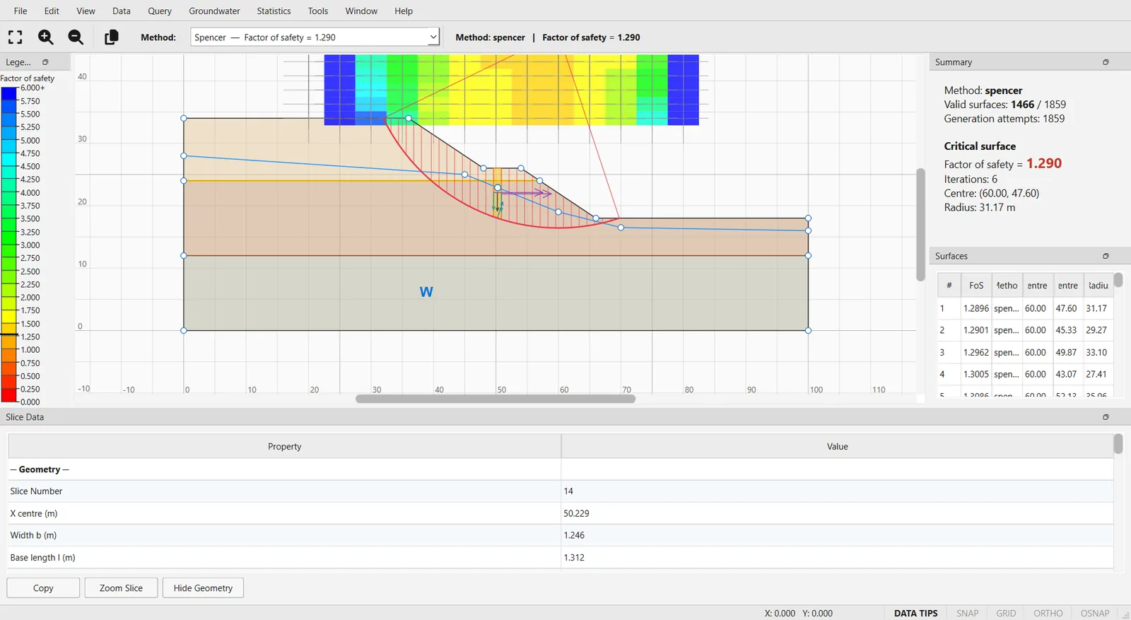
Critical and ranked surfaces, slice data, free-body diagrams, line of thrust, charts along the slope and reports.
Data sheet
Taken from the source code of version 0.1.235. If you find a difference between this page and the program, the program is right; let us know and we will correct the page.
- Analysis
- 2D limit equilibrium, plane strain
- Methods
- Ordinary, Bishop, Janbu simplified & corrected, Spencer, GLE / Morgenstern–Price, Lowe–Karafiath, Corps of Engineers #1 & #2
- Surfaces
- Circular, non-circular, composite, weak layers
- Searches
- Grid, slope, auto-refine, block, path, simulated annealing, particle swarm
- Strength models
- 22, from Mohr–Coulomb to generalised anisotropic
- Pore pressure
- Water table, piezometric lines, ru, grids, FE seepage, B̄, suction
- Groundwater FE
- Steady and transient, saturated and unsaturated, 6 permeability functions
- Probabilistic
- Monte Carlo, Latin hypercube, 7 distributions, sensitivity
- Supports
- 9 types, active or passive, back analysis
- Seismic
- Pseudo-static, yield acceleration, Newmark displacement
- Design codes
- Eurocode 7 DA1-C1, DA1-C2, DA2, DA3, custom
- Files
- .ogr (JSON), DXF in and out, PDF reports, CSV, HDF5 results
- Interfaces
- Desktop (PySide6), Python terminal and API, CLI, MCP server
- Languages
- English and Spanish interface
- Requirements
- Python 3.11 or newer
- Licence
- AGPL-3.0-or-later · no warranty
A suite of 5 265 tests
The tests compare results with published cases, closed-form solutions and analytic identities. We do not use stored outputs of the program as references, because a stored output would also preserve any error it contained.