Probabilistic analysis — OGR Slip2D documentation

A factor of safety is computed from parameters that are known only approximately. A probabilistic analysis describes some of them as random variables, samples them many times and reports how the factor of safety varies: its mean and spread, the probability that it falls below one and a reliability index. The sensitivity analysis, which sweeps one parameter at a time, is covered at the end of the chapter.

3.11.1Random variables#

A random variable names one input of the model (which parameter of which object) and attaches a distribution to it. The inputs that can be made random are:

any parameter of a material's strength model: $c'$ and $\phi'$ , and the parameters of every non-linear model (Section 3.5);
the unit weight and saturated unit weight of a material, its $r_u$ , its constant pore pressure, its $\phi^b$ and its air-entry value;
the hydraulic properties of a material that has them: saturated permeability, anisotropy ratio and angle, the parameters of the unsaturated functions, the saturated and residual water contents and the specific storage;
the magnitudes of distributed and line loads;
the seismic coefficients $k_h$ and $k_v$ ;
the position of the water table, as a vertical offset with mean zero that moves every vertex of the water table by the same amount.

Each variable is given by a mean $\mu$ , which starts at the current value of the parameter, a standard deviation $\sigma$ , and a relative minimum and maximum: distances below and above the mean. The variable is truncated to

a = \mu - \Delta_{min}, \qquad b = \mu + \Delta_{max}

which is how uncertainty is usually stated (‘10 kPa, give or take 4’). With a minimum distance smaller than the mean, it also keeps every sample physically possible: a friction angle truncated this way cannot come out negative. A new variable starts with $\sigma$ equal to 10 % of its mean and a range of 30 % of the mean on either side, or 0.1 and 0.3 in absolute terms when the mean is zero. A variable whose range is zero, or a normal or lognormal variable with no standard deviation, is not random and keeps its mean; the normal, lognormal, beta and gamma distributions all need a positive standard deviation.

In OGR Slip2D

Random variables are defined in Statistics → Random Variables, which lists every parameter of the model that can be sampled and plots the density of the one being edited. Each sample is written into a copy of the project, so the model itself is never changed by a statistical run. When a definition no longer matches the model (a material deleted since, for example), the run names the variable instead of leaving it out without warning.

Source: ogr_core/statistics/random_variables.py

3.11.2Distributions#

Seven distributions are available. Table 3.11.1 gives the density of each and how its parameters are obtained from the inputs; $a$ and $b$ are the bounds of Eq. (3.11.1).

Table 3.11.1 The seven distributions of OGR Slip2D: the density

f(x)

before truncation, and how each is parameterised from the mean

\mu

, the standard deviation

\sigma

and the bounds

a,\ b

Distribution	Density	Parameters
Normal	$\dfrac{1}{\sigma\sqrt{2\pi}}\,e^{-(x-\mu)^2/2\sigma^2}$	$\mu,\ \sigma$ as entered
Uniform	$\dfrac{1}{b - a}$ on $[a,\ b]$	bounds only; $\sigma$ is not used
Triangular	$\dfrac{2(x - a)}{(b - a)(c - a)}$ for $x < c$ , $\dfrac{2(b - x)}{(b - a)(b - c)}$ for $x \ge c$	apex $c = \mu$ ; $\sigma$ is not used
Beta	$\dfrac{(x - a)^{p-1}(b - x)^{q-1}}{B(p,q)\,(b - a)^{p+q-1}}$ on $[a,\ b]$	$m = \frac{\mu - a}{b - a}$ , $v = \left(\frac{\sigma}{b - a}\right)^2 \le 0.999\,m(1 - m)$ , $k = \frac{m(1 - m)}{v} - 1$ , $p = m k$ , $q = (1 - m)k$
Exponential	$\lambda\,e^{-\lambda x}$ , $x \ge 0$	$\lambda = 1/\mu$ ; $\sigma$ is not used
Lognormal	$\dfrac{1}{x\,\sigma_{\ln}\sqrt{2\pi}}\,e^{-(\ln x - \mu_{\ln})^2/2\sigma_{\ln}^2}$	$\sigma_{\ln}^2 = \ln\!\left(1 + \sigma^2/\mu^2\right)$ , $\mu_{\ln} = \ln\mu - \sigma_{\ln}^2/2$
Gamma	$\dfrac{x^{k-1}e^{-x/\theta}}{\Gamma(k)\,\theta^{k}}$	$\theta = \sigma^2/\mu$ , $k = \mu^2/\sigma^2$

The lognormal and gamma distributions are parameterised by the mean and standard deviation of the variable itself, which is what a user knows, not of its logarithm or of the shape and scale; the beta distribution is fitted by moments on $[a,\ b]$ , so it keeps $\mu$ and $\sigma$ whenever that standard deviation is attainable on the range (its shape parameters are kept at or above $10^{-3}$ ). For the uniform and triangular distributions the mean only places the bounds and, for the triangle, its apex: with an asymmetric range the mean of the samples is not $\mu$ . With $\mu = 10$ , $\Delta_{min} = 6$ and $\Delta_{max} = 10$ , the uniform samples have a mean of 12 and the triangular ones of 11.33 (Figure 3.11.1).

Figure 3.11.1 Densities of the seven distributions for one variable with

\mu = 10

\sigma = 3

and a relative minimum and maximum of 6 and 10, that is truncated to [4, 20], as the sampler draws them: each curve is the program's own density divided by

F(b) - F(a)

(Eq. (3.11.2)). All panels share one vertical scale. Computed with OGR Slip2D 0.1.235.

3.11.3Truncation#

The range is imposed by inverse-CDF remapping, not by rejection. A uniform variate $u \in [0, 1)$ is mapped onto the part of the cumulative distribution that lies between the bounds, and inverted:

x = F^{-1}\!\Big(F(a) + u\,\big[F(b) - F(a)\big]\Big)

where

$F,\ F^{-1}$: cumulative distribution function of the untruncated distribution, and its inverse

Every sample lies in $[a,\ b]$ (it is also clipped to it against round-off), the density inside the range is $f(x)/[F(b) - F(a)]$ , and, unlike rejection, the mapping keeps the stratification of Latin hypercube sampling intact: every stratum of $u$ still produces exactly one sample.

3.11.4Sampling#

Monte Carlo sampling (Metropolis & Ulam, 1949) draws every uniform variate independently. Latin hypercube sampling (McKay, Beckman & Conover, 1979) divides $[0, 1)$ into $N$ equal strata and draws one variate in each,

u_i = \dfrac{i + U_i}{N}, \qquad i = 0, 1, \ldots, N - 1, \qquad U_i \sim \mathcal{U}[0, 1)

then shuffles them independently for every variable. Each variable thus covers its whole distribution evenly with $N$ samples, while the pairing between variables stays random (Figure 3.11.2). An option shares one stratification among all the variables instead: sample $i$ then falls in the same stratum of every variable, so they all move together. That answers a different question (what happens if every parameter is unfavourable at once) and usually widens the spread of the factor of safety; it has no meaning for Monte Carlo sampling, which has no strata.

The random stream is pseudo-random from a seed, so that the same model and seed give the same samples, or random, seeded from the clock, which is a way of checking that a conclusion does not depend on one particular seed.

Figure 3.11.2 Ten samples of two independent uniform variables drawn by Monte Carlo sampling (left) and by Latin hypercube sampling (right) with the sampler of OGR Slip2D and seed 10116. In the Latin hypercube every row and every column of the 10 × 10 grid holds exactly one sample.

3.11.5Correlation between cohesion and friction angle#

A variable can be declared correlated with another one, with a coefficient $\rho$ between −1 and 1. The intended use is the cohesion and friction angle of a Mohr–Coulomb material, where a negative coefficient is the usual case. OGR Slip2D imposes the correlation after sampling, by reordering in the manner of Iman & Conover (1982): both variables keep their sampled values, and so their distributions, exactly; only the pairing changes. With $r_i$ the rank of the $i$ -th value of the reference variable among its $N$ values,

z_i = \Phi^{-1}\!\left(\dfrac{r_i - \frac12}{N}\right), \qquad t_i = \rho\,z_i + \sqrt{1 - \rho^2}\;\varepsilon_i

where

$\Phi^{-1}$: inverse of the standard normal distribution
$\varepsilon_i$: independent standard normal numbers

and the sorted values of the correlated variable are reassigned so that their ranks follow the ranks of $t$ . Working with normal scores of the ranks rather than with the ranks themselves is what brings the achieved coefficient close to the requested one, which it matches only approximately. The scores used are $\Phi^{-1}((r - \frac12)/N)$ , a variant of the van der Waerden scores $\Phi^{-1}(r/(N + 1))$ of Iman and Conover; the two differ only in the plotting position.

In OGR Slip2D

The analysis is configured in Analysis → Project Settings → Statistics, with Probabilistic analysis, Analysis type (Global Minimum by default), Sampling method (Monte Carlo by default) and Number of samples (1000), and in Random Numbers, with Generation (pseudo-random by default), Seed (10116) and the shared Latin hypercube stratification (off). The same seed also drives the searches that draw surfaces at random. The correlation of a variable is set beside its distribution, in Statistics → Random Variables.

Source: ogr_core/statistics/distributions.py · ogr_core/project/settings.py

3.11.6Global minimum and overall slope#

Global minimum, the default, first runs the deterministic analysis to locate the critical surface of each method, then re-evaluates that surface for every sample. The circle (or polyline) is fixed, but each sample resolves its own sliding mass on it, with the search settings of the deterministic run, so a sample costs one limit-equilibrium solve per method. Each method keeps its own critical surface.

Overall slope repeats the whole search for every sample, so the position of the critical surface is not assumed: the factor of safety of a sample is the minimum its search finds. This costs a full search per sample. The run also accumulates the factors of every surface it evaluates and reports the critical probabilistic surface: the surface with the highest probability of failure among those evaluated at least five times, ties broken by the lower reliability index, which need not be the deterministic critical surface. Surfaces are matched across samples by their geometry rounded to 0.5 m.

In both types a sample whose surface cannot be solved, or is inadmissible (Section 3.3), has no factor of safety: it is left out of the statistics and counted by cause, and the run warns about the loss (in a global-minimum run, once more than 20 % of the samples are lost).

In OGR Slip2D

With a design standard on, the program prepares every sample like the deterministic analysis: the sampled values are written into a copy of the model and that copy is then factored, so the statistics describe the over-design factor and its probability of falling below one (Section 3.12).

Source: ogr_core/statistics/probabilistic.py · ogr_slip2d/analysis_runner.py

3.11.7Probability of failure and reliability index#

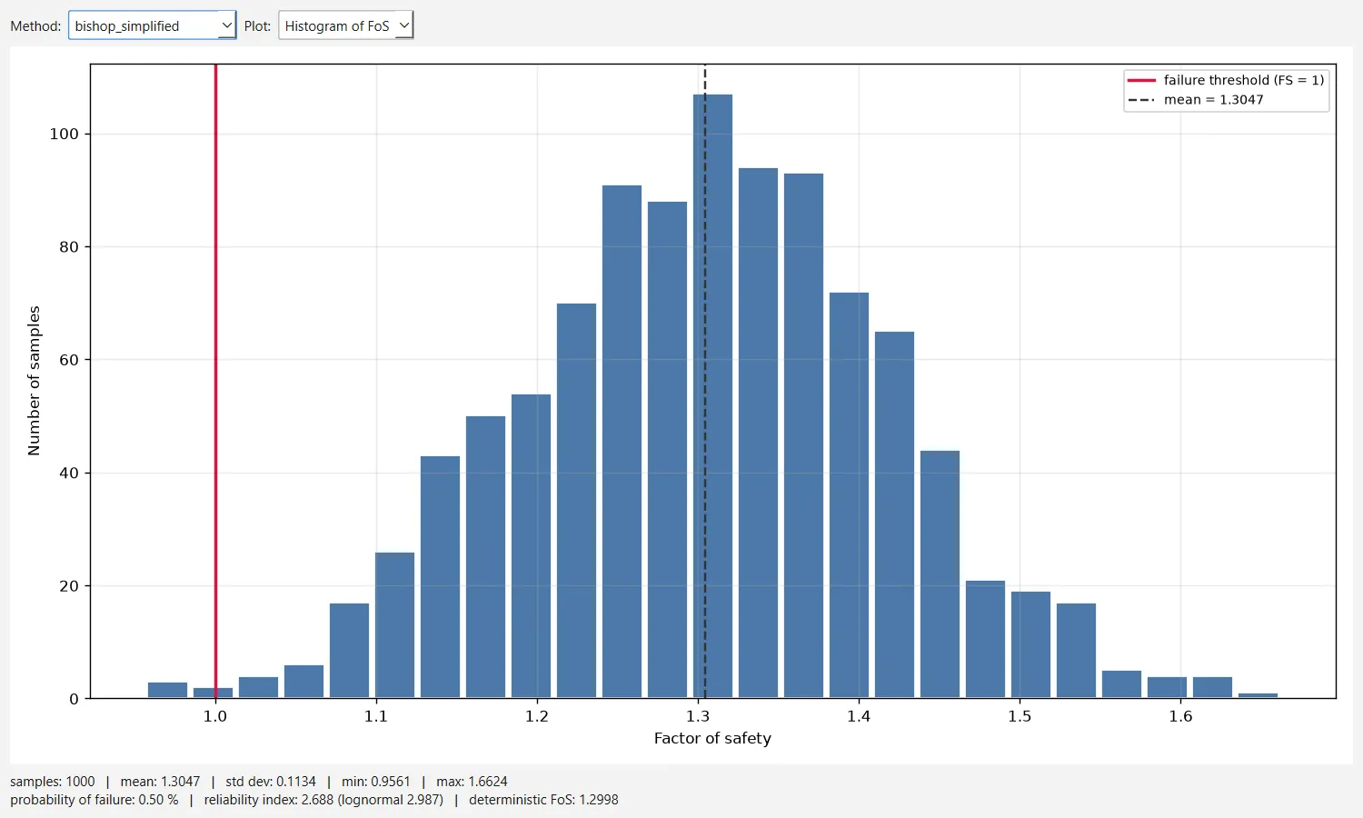
The probability of failure is the fraction of valid samples whose factor of safety is below one:

P_F = \dfrac{n(F < 1)}{N_v}

where

$N_v$: number of samples that produced a valid, admissible factor of safety
$n(F < 1)$: number of them with $F$ strictly below one

The reliability index measures the distance from the mean factor of safety to failure in standard deviations (Cornell, 1969). OGR Slip2D reports it in two forms:

\beta = \dfrac{\mu_F - 1}{\sigma_F}

\beta_{\ln} = \dfrac{\mu_{\ln F}}{\sigma_{\ln F}}

where

$\mu_F,\ \sigma_F$: mean and standard deviation of the sampled factors of safety, the standard deviation with $N_v - 1$ in the denominator
$\mu_{\ln F},\ \sigma_{\ln F}$: the same statistics of $\ln F$ , over the positive factors of safety

The lognormal form applies the same definition to $\ln F$ , for which failure is $\ln F = 0$ ; it often describes a factor of safety better, since a factor of safety cannot be negative. A sampling with no scatter gives $\beta = \pm\infty$ . The probability of failure itself makes no assumption about the shape of the distribution of $F$ .

Figure 3.11.3 Schematic histogram of 1000 factors of safety, drawn with the program's sampler from a lognormal distribution with mean 1.30 and standard deviation 0.20 (seed 10116). The shaded bars,

F < 1

, make up

P_F = 0.047

; with

\mu_F = 1.30

and

\sigma_F = 0.198

\beta = 1.51

and

\beta_{\ln} = 1.65

, as the program computes them from these samples.

The Statistics window of OGR Slip2D: histogram of 1 000 sampled factors of safety of the two-layer slope, with the failure threshold, the mean and the summary line — Figure 3.11.4 The Statistics window after a run on the two-layer slope of the quick start (example 4), with the cohesion of the clay (normal, mean 12 kPa, standard deviation 3 kPa), its friction angle (24°, 2.4°) and the friction angle of the silty sand (32°, 2°) as random variables, each truncated at three standard deviations, and 1 000 Monte Carlo samples on the deterministic critical surface. Bishop: $\mu_F = 1.305$ , $\sigma_F = 0.113$ , $P_F = 0.5\,\%$ (five samples below 1), $\beta = 2.69$ and $\beta_{\ln} = 2.99$ .

3.11.8Convergence#

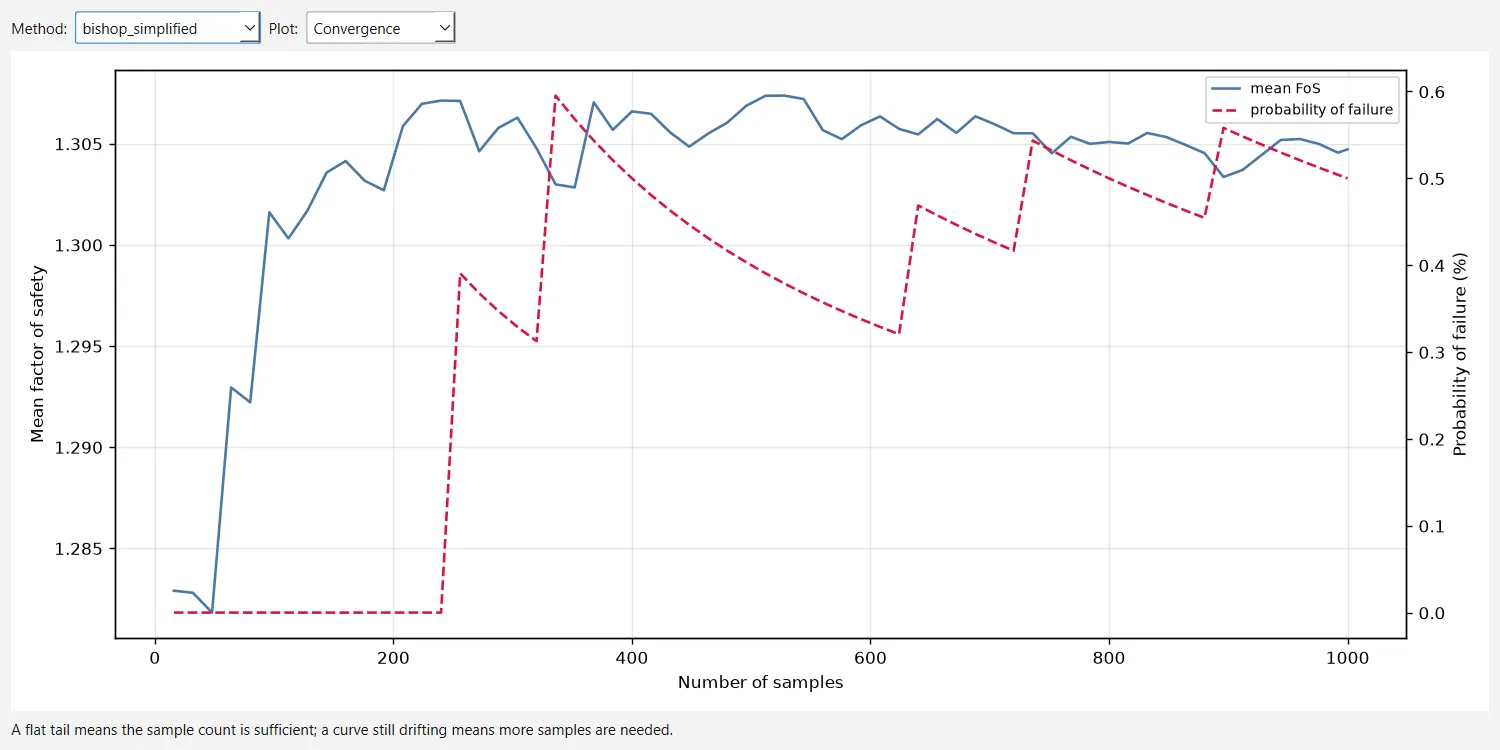
The estimates settle as the number of samples grows. OGR Slip2D records the running mean factor of safety and the running probability of failure along the sequence of samples, at about 50 points (every $N/50$ samples, and at the last one). That is the convergence plot of a run: a mean or a probability that is still moving at the last sample calls for more samples. A small probability of failure needs many samples to be estimated at all, since it is a count of rare events.

Convergence plot of the Statistics window: the running mean factor of safety and the running probability of failure against the number of samples — Figure 3.11.5 Convergence of the run of Figure 3.11.4. The running mean stays within 0.003 of its final value from about 300 samples on; the probability of failure, five failing samples in 1 000, still jumps at every new failure. An estimate of a probability of this order needs many more samples.

3.11.9Sensitivity analysis#

A sensitivity analysis is not probabilistic: the shape of the distributions plays no part, and only the minimum and maximum of each variable are used. Each variable is swept, one at a time, across its range divided into $n$ equal intervals,

x_j = a + (b - a)\,\dfrac{j}{n}, \qquad j = 0, 1, \ldots, n

and the factor of safety is recomputed on the critical surface of each method at every value, with all the other parameters at their values in the deterministic model. With the default $n = 50$ that is 51 evaluations per variable and method. The variables are ranked by the span of the factor of safety over their range; for each, the program also reports where the curve crosses a target factor of safety, by linear interpolation between the two values that bracket it, and the horizontal axis can be expressed as a percentage of each range, so that variables with different units share one plot. Values at which the surface has no admissible factor of safety are left out of the curve.

In OGR Slip2D

Sensitivity analysis and the number of Sensitivity intervals (50 by default) are on the Analysis → Project Settings → Statistics page. The sweep uses the same random variables as the probabilistic analysis, and with a design standard on each swept model is factored like the deterministic one.

Source: ogr_core/statistics/sensitivity.py

3.11.10References#

Cornell, C.A. (1969). A probability-based structural code. Journal of the American Concrete Institute, 66(12), 974–985.
Iman, R.L. & Conover, W.J. (1982). A distribution-free approach to inducing rank correlation among input variables. Communications in Statistics — Simulation and Computation, 11(3), 311–334.
McKay, M.D., Beckman, R.J. & Conover, W.J. (1979). A comparison of three methods for selecting values of input variables in the analysis of output from a computer code. Technometrics, 21(2), 239–245.
Metropolis, N. & Ulam, S. (1949). The Monte Carlo method. Journal of the American Statistical Association, 44(247), 335–341.