Instead of taking the pore pressures of a slope as input, OGR Slip2D can compute them by solving, with finite elements on a mesh of the model, the equations of groundwater flow in saturated and unsaturated soil, steady or transient. The sections below give the equations and the numerical choices made to solve them (element, mesh, boundary conditions, iteration on seepage faces, permeability functions and integration in time); how the resulting field reaches the limit-equilibrium analysis is described at the end and in Section 3.6.
3.7.1Governing equations#
Water moves through the pores under gradients of total head. With the pressure head , the total head at elevation is
The discharge per unit area, or Darcy velocity, follows the law of Darcy (1856), extended to unsaturated soil by letting the conductivity depend on the suction:
where
- Darcy velocity (m/s)
- saturated conductivity tensor of the material (m/s), Section 3.7.2
- relative permeability, 1 in saturated soil (—), Section 3.7.7
- suction head where the pressure head is negative (m)
Conservation of mass (the net outflow of a volume equals the rate at which it loses stored water) gives the equation of Richards (1931), written here in its mixed form, with the volumetric water content as the stored quantity:
In a steady state the left-hand side vanishes:
With everywhere the equation is linear and describes saturated, confined flow; with a permeability function the conductivity depends on the solution and the equation has to be solved iteratively (Section 3.7.6). The same equation holds above and below the phreatic surface, so the free surface is not a boundary of the problem but the line of its solution.
Heads are in the length unit of the model; the solver itself does not depend on the unit, as long as the conductivities and the times of a transient analysis use the same one (for instance m/s and seconds). Pore pressures are , with the pore-fluid unit weight of the project.
Source: ogr_fem2d/solvers/seepage.py3.7.2Anisotropic conductivity#
Each material has a saturated permeability , which is its major principal conductivity , a ratio and the angle of measured from the axis. The tensor in the axes of the model is the rotation of the principal one:
It is symmetric and positive definite for . In the unsaturated zone the whole tensor is multiplied by , so the anisotropy ratio and its direction are kept.
Groundwater → Define Hydraulic Properties… sets Saturated permeability Ks (default ), K2 / K1 (default 1) and K1 angle (deg from +X) (default 0). A material with no hydraulic properties is solved with these defaults, and the message after Compute Groundwater names it.
Source: ogr_core/hydraulic/hydraulic_properties.py · ogr_slip2d/transient_stability.py3.7.3Linear triangles#
The model is divided into three-node triangles with linear shape functions . The Galerkin form of Eq. (3.7.4) on one element gives its conductance matrix. Because the gradients of linear shape functions are constant over the element, the matrix is exact in closed form, without numerical integration (Bathe & Khoshgoftaar, 1979):
where
- area of the element (m²)
- relative permeability of the element (—)
- cyclic permutation of the three nodes, numbered anticlockwise
Assembly gives the linear system , where holds the nodal flows of the flow conditions. The head is linear within each element, so the velocity of Eq. (3.7.2) is constant in it. The relative permeability of an element is evaluated at the mean of the pressure heads of its three nodes, which for a linear field is the value at its centroid.
The system is solved with a sparse direct solver. Prescribed heads are imposed by elimination, which keeps the reduced system symmetric. A problem with no prescribed head anywhere is singular (the head is defined only up to a constant) and is reported as an error.
Source: ogr_fem2d/solvers/seepage.py · ogr_fem2d/mesh/mesh.py3.7.4Meshing#
The mesh is generated region by region over the material regions of the model, so that no element straddles a material boundary and the material of every element is exact:
- Every edge of every region is divided into segments of about the target size . All boundary nodes go through one registry keyed by their coordinates, so an edge shared by two regions receives the same nodes in both: the mesh is conforming across material interfaces without any stitching afterwards.
- Each region is filled with interior points on a staggered, near-equilateral lattice of spacing , kept at least from its outline, and its points are joined by a Delaunay triangulation. Triangles whose centroid falls outside the region, or inside a hole of it, are discarded.
- Triangles with a smallest angle below 25° receive their circumcentre as a new point and the region is triangulated again, up to three times (Chew, 1989; Ruppert, 1995). A circumcentre outside the region, closer than to its outline or closer than to an existing point is not inserted, which keeps the refinement finite.
Unless a size is given, is the side of the equilateral triangles that would fill the area of the model with the requested number of elements :
Groundwater → Mesh → Generate FE Mesh… asks for the approximate number of elements, 1000 by default (20 to 200 000). The minimum angle (25°) and the number of refinement passes (3) can be changed from the scripting interfaces. A lens is meshed once, as a hole in the region around it. A new mesh discards the boundary conditions and fields of the previous one, which are tied to its node numbers.
Source: ogr_fem2d/mesh/generator.py · ogr_fem2d/mesh/mesh.py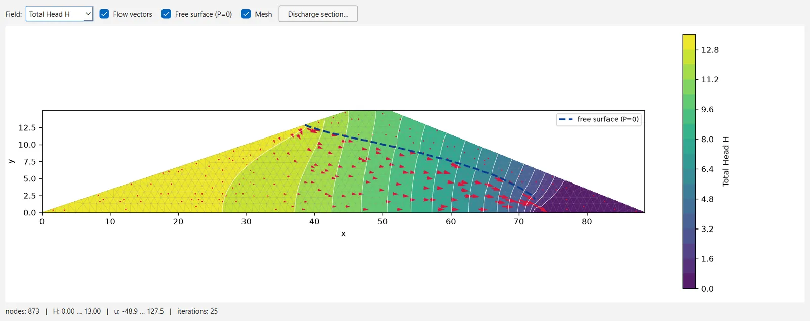
3.7.5Boundary conditions#
Six kinds of condition can be applied to the nodes of the boundary (Table 3.7.1). Three prescribe the head, two prescribe a flow, and the sixth is the condition of a possible seepage face.
| Condition | Identifier | Kind | Prescribes |
|---|---|---|---|
| Total Head | total_head | head | equal to the value |
| Pressure Head | pressure_head | head | , with equal to the value |
| Zero Pressure | zero_pressure | head | |
| Nodal Flow Rate | nodal_flow | flow | a flow per unit thickness of the model at the node |
| Infiltration | infiltration | flow | a flux per unit length of boundary, given to the two nodes of each edge as , the consistent load of a linear element |
| Unknown (P=0 or Q=0) | unknown | unilateral | either with water leaving, or no flow (Section 3.7.6) |
When a mesh is generated, every boundary node receives a default condition. The nodes on the left, right and bottom edges of the bounding box of the model get a zero nodal flow, which makes those edges impermeable; all the others, including the ground surface and the slope face, get Unknown. The defaults prescribe no head, so a head has to be assigned somewhere before the problem can be solved.
A reservoir is assigned by its level and by the side it stands on. The program prescribes a total head equal to the level on the wetted perimeter, which it finds by walking along the boundary from the vertical edge on that side, up the ground surface, for as long as the ground stays at or below the level. The walk stops at the first node above the level and never enters the base or the far edge of the model. The submerged part of the vertical edge is included by default. Lowering a reservoir is the same assignment with a lower level. Figure 3.7.2 shows these conditions on an embankment and the solution the program computes with them. A nodal-flow condition can also be marked as a possible seepage face, which adds its node to the switching of Section 3.7.6.
Groundwater → Set Boundary Conditions… assigns a condition to a side of the model (Left edge, Right edge, Bottom edge, Ground surface) or places a reservoir on the left or the right; Restore defaults brings back the conditions above. The scripting interfaces can also address individual nodes and the stretch of boundary along a polyline. A set of conditions belongs to one mesh: a set that names nodes the current mesh does not have is replaced by the defaults.
Source: ogr_fem2d/solvers/seepage.py · ogr_fem2d/solvers/bc_targets.py3.7.6Picard iteration and seepage faces#
Two non-linearities are resolved together: the conductivity depends on the suction, and each Unknown node has to settle as either seepage face or impermeable. The program starts from the linear solution with and every Unknown node impermeable. Then, at each iteration , it evaluates of every element from the current heads, solves the linear system with the nodes currently on the seepage face held at , and relaxes the update:
where
- heads of the linear solution with the conductivities of iterate
- relaxation factor, between 0.05 and 1 (—)
Under-relaxation keeps the iteration from oscillating when the permeability function is steep, as it is in sands.
The seepage face#
Where the free surface meets an exposed face, water leaves the model at atmospheric pressure. The extent of that seepage face is not known beforehand, so the Unknown nodes obey a unilateral condition: either with water flowing out, or no flow with . The program finds it by nodal switching (Neuman, 1973; Bathe & Khoshgoftaar, 1979): a free node whose pressure head becomes positive is held at , and a held node whose nodal reaction shows water entering the model is released to no flow. Two tolerance bands prevent the switching from chattering (a pressure head of 2 % of the element size and a reaction of times the largest reaction of the first solution), and a node that has switched 25 times is frozen.
The iteration has converged when the largest change of head is below the tolerance and no node has switched. The final state is then checked against the unilateral condition itself: if any Unknown node still violates it, the run is reported as not converged, whatever stopped the loop. The mesh never moves; the free surface is traced afterwards as the line where the pressure head changes sign.
Groundwater → Compute Groundwater solves the steady problem with , at most 200 iterations and a tolerance of m on the head; a run that does not converge is reported with its reason. The free surface drawn by Interpret Groundwater is the highest change of sign of the pressure head on each of a series of vertical lines.
Source: ogr_fem2d/solvers/seepage.py · ogr_slip2d/transient_stability.py3.7.7Permeability functions#
The relative permeability of each material is one of seven functions of the suction. Two of them are written in suction head , in metres of water, and the others in matric suction , in kPa; the solver gives each function its own variable, with . All equal 1 at zero suction and are limited below by , so that the conductance matrix never becomes singular in very dry zones. Table 3.7.2 lists the functions with their default parameters, and Figure 3.7.3 plots them.
Constant. : the material conducts as if saturated at any suction, and the problem is linear if every material uses it.
Simple. A function of the program, not taken from the literature: the permeability falls log-linearly by orders of magnitude over a suction range and stays constant beyond it,
with = (100 kPa, 1) for the general soil type, (10 kPa, 4) for sand, (50 kPa, 3) for silt, (1500 kPa, 2) for clay and (100 kPa, 3) for loam.
Brooks–Corey. From the power-law retention curve of Brooks & Corey (1964), with the pore-size index and the bubbling pressure :
Fredlund–Xing. The relative permeability takes the form of the soil–water characteristic curve of Fredlund & Xing (1994), normalised and without the correction factor of the original equation:
Gardner. The function of Gardner (1958), in suction head:
van Genuchten. The closed form of van Genuchten (1980), obtained from his retention curve with the conductivity model of Mualem (1976), in suction head:
The closed form holds for . The program allows to be released, and then applies the same expression with the value given.
User defined. A table of points . The relative permeability is the tabulated permeability divided by that of the first point, interpolated linearly in suction and logarithmically in permeability; it is 1 below the first suction and keeps the last ratio beyond the last one.
| Function | Identifier | Variable | Parameters (default) |
|---|---|---|---|
| Constant | constant | — | — |
| Simple | simple | (kPa) | soil type (general) |
| Brooks–Corey | brooks_corey | (kPa) | , kPa |
| Fredlund–Xing | fredlund_xing | (kPa) | kPa, , |
| Gardner | gardner | (m) | m−n, |
| van Genuchten | van_genuchten | (m) | m−1, , |
| User Defined | user_defined | (kPa) | table of at least two points |
The function is chosen in Groundwater → Define Hydraulic Properties…; Plot draws it in its own variable, and Pick loads representative values for Brooks–Corey, Fredlund–Xing, Gardner and van Genuchten (the van Genuchten textures are those of Carsel & Parrish, 1988, converted to m−1). For a User Defined table the conductivity is times the tabulated ratio.
Source: ogr_core/hydraulic/permeability_models.py · ogr_core/hydraulic/hydraulic_properties.py3.7.8Transient analysis#
A transient analysis follows the field in time from an initial state, through stages whose boundary conditions may differ: a reservoir drawn down, a period of rainfall. It integrates Eq. (3.7.3) in mixed form, with the stored water as the accumulated quantity. That form keeps the mass balance of the discrete solution, whereas the form in which is replaced by accumulates errors of mass balance (Celia, Bouloutas & Zarba, 1990).
Storage#
The stored water is one function of the pressure head that joins the capillary storage of the unsaturated zone and the elastic storage of the saturated one:
where
- saturated and residual volumetric water contents (—)
- specific storage of the saturated soil (m−1)
- specific moisture capacity, the slope of the retention curve (m−1)
Below the water table the water content is constant; without the specific storage the transient equation would reduce there to the steady one. Whatever its permeability function, the water content of every material follows the retention curve of van Genuchten (1980), with the material's , and (Figure 3.7.4):
Integration in time#
Time is integrated with the implicit (backward) Euler method, which is unconditionally stable. Each step is solved by the modified Picard iteration of Celia, Bouloutas & Zarba (1990), which linearises the storage about the current iterate but carries the change of stored water explicitly:
where
- previous time level and current Picard iterate of the new one
- lumped (diagonal) mass matrix: each node receives one third of the area of every element it belongs to (m²)
- diagonal of nodal storage coefficients at the iterate (m−1)
- stored water at the nodes at the iterate and at the previous time level (—)
- conductance matrix with the relative permeabilities of the iterate
- time step
The update is relaxed as in the steady case, the switching of the seepage face is applied at every iteration of every step, and a step has converged when the largest change of head is below the tolerance and no node has switched.
Stages and time steps#
Each stage ends at its time and may have its own boundary conditions; a stage without them uses the current ones. A stage is divided into equal steps, either a fixed number of them or a number chosen so that a wetting front cannot cross much more than one element per step:
where
- target element size of the mesh (m)
- largest saturated permeability in the model
- smallest storage coefficient of the materials at a pressure head of −1 m, and never more than 1 (m−1)
The initial state is the steady solution for the initial boundary conditions: those stored with the transient analysis, or the current ones if it stores none. A stage of zero duration reports the state it inherits.
The stages (time, label, Calculate SF and their own conditions) are defined in Groundwater → Transient Groundwater…. Analysis → Project Settings → Transient sets the tolerance ( m), the maximum number of Picard iterations per step (30) and the number of time steps per stage (Auto by default). The transient solver relaxes with , also in its initial steady state, which may take up to 200 iterations. Each node takes the storage parameters of one of the elements that share it, the first in the element list. The stored water and its change are recorded for every stage as a check of the mass balance. The transient analysis, excess pore pressure and rapid drawdown are mutually exclusive.
Source: ogr_fem2d/solvers/seepage.py · ogr_core/hydraulic/hydraulic_properties.py · ogr_slip2d/transient_stability.py · ogr_core/project/settings.py3.7.9Coupling to the stability analysis#
The nodal pore pressures reach the limit-equilibrium analysis through the materials of type fem, interpolated at the base midpoint of each slice (Eq. (3.6.9)); negative values pass through the treatment of unsaturated strength (Section 3.6.9). The boundary conditions define where water stands on the slope: there is ponded water wherever a prescribed total head or pressure head exceeds the elevation of its node (Section 3.6.7).
In a transient analysis, every stage flagged Calculate SF is analysed with the project's methods and search, with the field of that stage and with the conditions that produced it, so that a stage of a drawdown carries neither the pore pressures nor the weight of the reservoir it has emptied. The result is a history of the factor of safety (Section 3.8.7).
The factors of safety of each stage are kept with its result and shown in Interpret Groundwater. If no material is of type fem, the stage factors are not computed and a warning explains why.
3.7.10Verification#
The solver is checked against closed-form solutions and identities (Section 4.3):
- one-dimensional confined flow, where the head is linear and the discharge follows Darcy's law;
- a patch test with a fully anisotropic tensor (), in which a uniform head gradient and its Darcy velocity are reproduced exactly;
- layered soils, whose equivalent conductivity is the harmonic mean of the layers for flow across them and the arithmetic mean for flow along them, with the flow balanced across a contrast of permeability of 100;
- the discharge through a rectangular dam on an impervious base, which has an exact closed form and is approached as the permeability function is made sharper, with the free surface leaving the downstream face above the tailwater;
- the response of a confined aquifer to a sudden change of head, which follows the complementary error function, and the transient solution at long times, which must reproduce the steady one;
- the retention curve and its derivative.
The permeabilities and boundary conditions of a seepage analysis are usually uncertain by more than its numerical error. Compare the computed water levels with piezometer readings where they exist, and check how sensitive the factor of safety is to the permeability contrasts that control the free surface.
3.7.11References#
- Bathe, K.J. & Khoshgoftaar, M.R. (1979). Finite element free surface seepage analysis without mesh iteration. International Journal for Numerical and Analytical Methods in Geomechanics, 3(1), 13–22.
- Brooks, R.H. & Corey, A.T. (1964). Hydraulic Properties of Porous Media. Hydrology Paper 3, Colorado State University, Fort Collins.
- Carsel, R.F. & Parrish, R.S. (1988). Developing joint probability distributions of soil water retention characteristics. Water Resources Research, 24(5), 755–769.
- Celia, M.A., Bouloutas, E.T. & Zarba, R.L. (1990). A general mass-conservative numerical solution for the unsaturated flow equation. Water Resources Research, 26(7), 1483–1496.
- Chew, L.P. (1989). Guaranteed-Quality Triangular Meshes. Technical Report TR 89-983, Department of Computer Science, Cornell University, Ithaca.
- Darcy, H. (1856). Les fontaines publiques de la ville de Dijon. Victor Dalmont, Paris.
- Fredlund, D.G. & Xing, A. (1994). Equations for the soil-water characteristic curve. Canadian Geotechnical Journal, 31(4), 521–532.
- Gardner, W.R. (1958). Some steady-state solutions of the unsaturated moisture flow equation with application to evaporation from a water table. Soil Science, 85(4), 228–232.
- Mualem, Y. (1976). A new model for predicting the hydraulic conductivity of unsaturated porous media. Water Resources Research, 12(3), 513–522.
- Neuman, S.P. (1973). Saturated-unsaturated seepage by finite elements. Journal of the Hydraulics Division, ASCE, 99(HY12), 2233–2250.
- Richards, L.A. (1931). Capillary conduction of liquids through porous mediums. Physics, 1(5), 318–333.
- Ruppert, J. (1995). A Delaunay refinement algorithm for quality 2-dimensional mesh generation. Journal of Algorithms, 18(3), 548–585.
- van Genuchten, M.Th. (1980). A closed-form equation for predicting the hydraulic conductivity of unsaturated soils. Soil Science Society of America Journal, 44(5), 892–898.