Quick start: your first model — OGR Slip2D documentation

This tutorial builds the slope on the home page from an empty project: a 16 m slope with a mid-height bench, three soils and a water table, analysed with three methods. It takes about fifteen minutes and goes through the usual steps of an analysis. The model is also available ready-made: ej01-two-layer-slope.ogr.

Figure 1.2.1 The model at the end of the tutorial: silty sand over clay over dense gravel, a water table, and the critical Spencer circle among the minimum surfaces of every grid centre.

1.2.1The problem#

All coordinates are in metres, with $x$ to the right and $y$ up. The ground falls from left to right: crest at $y = 34$ , a 6 m wide bench at $y = 26$ and the toe at $y = 18$ ; both faces are inclined 1V:1.5H.

Table 1.2.1 Materials of the tutorial. All three use the water table for their pore pressure.

Material	Layer	c′ (kPa)	φ′ (°)	γ (kN/m³)
Silty sand	above y = 24	5	32	19.0
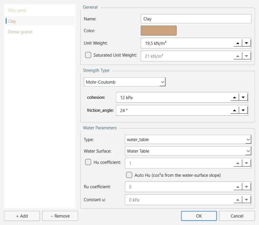
Clay	between y = 12 and 24	12	24	19.5
Dense gravel	below y = 12	0	40	21.0

1.2.2Start a project and set it up#

Start the program (ogr-slip2d). It opens with an empty project; if not, use File → New Project (Ctrl+N).
Open Analysis → Project Settings… (Ctrl+J). On the General page keep metric units with stresses in kPa, and set the failure direction to left to right: the ground falls to the right.
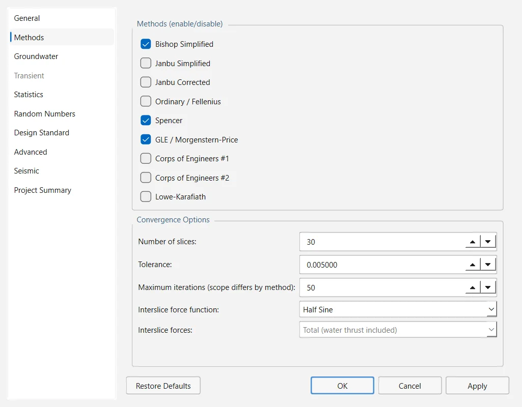
On the Methods page enable Bishop Simplified, Spencer and GLE / Morgenstern-Price, and set the number of slices to 30.

The Methods page of the Project Settings dialog with three methods enabled and 30 slices — Figure 1.2.2 Project Settings, Methods page.

1.2.3Draw the boundaries#

Boundaries can be drawn with the mouse, but typing the coordinates is exact. With a drawing tool active, type each vertex in the Enter X,Y field at the right of the status bar and press Enter; finish the boundary with Enter on an empty field, or from the right-click menu.

Boundaries → Add External Boundary (Ctrl+1): 0,0 · 100,0 · 100,18 · 66,18 · 54,26 · 48,26 · 36,34 · 0,34. The external boundary closes itself.
Boundaries → Add Material Boundary (Ctrl+2): 0,24 · 57,24, the contact between sand and clay, which ends on the lower face.
Again for the clay–gravel contact: 0,12 · 100,12.
Boundaries → Add Water Table (Ctrl+3): 0,28 · 45,25 · 60,19 · 70,16.5 · 100,16.

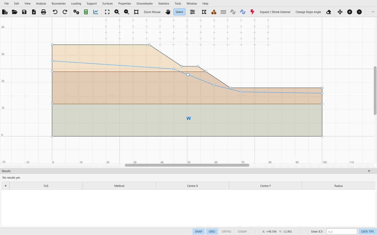
The canvas with the external boundary, two material boundaries and the water table — Figure 1.2.3 External boundary, two material boundaries and the water table. Each closed region between boundaries will receive one material.

A water table has to be assigned

A water table only produces pore pressure in the materials that use it. When you finish drawing it, the program offers to assign it; if you skip that step, do it later with Properties → Assign Water Surface….

1.2.4Define and assign the materials#

Properties → Define Materials…: create the three materials of Table 1.2.1, with strength type Mohr-Coulomb and pore pressure from the water table.
Properties → Assign Materials: pick a material and click inside its region; repeat for the three layers.

The Define Materials dialog with Mohr-Coulomb parameters — Figure 1.2.4 Define Materials. The strength parameters shown depend on the strength type chosen.

Regions left unassigned

A region nobody assigns takes the first material of the list. Check the colours on the canvas before computing; with DATA TIPS on in the status bar, hovering over a region shows its material.

1.2.5Choose the slip surfaces#

The default search is a grid of circle centres. Surfaces → Auto Grid places a grid above the slope sized from the geometry; Surfaces → Surface Options… shows the surface type (circular) and the search method (grid). For each centre, the program tries a set of radii between the shortest circle that reaches the slope and the longest that stays within the slope limits.

1.2.6Compute#

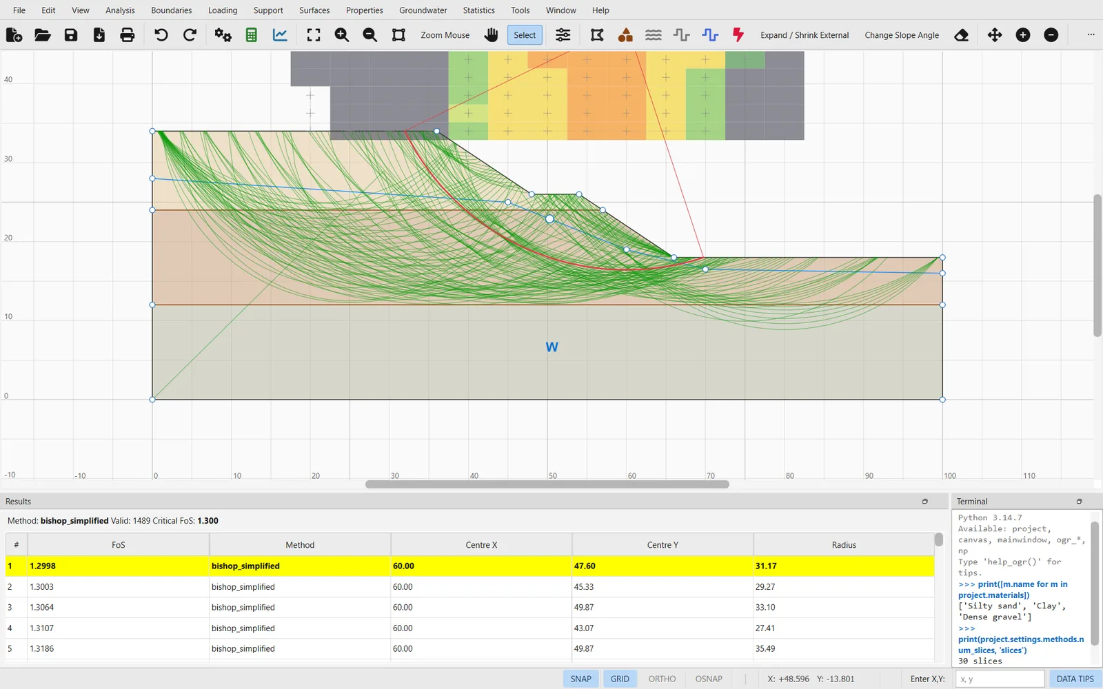
Analysis → Compute (Ctrl+T) runs the search for each enabled method in the background, with a progress dialog and a cancel button. When it finishes, the Results dock lists the lowest surfaces and the canvas draws them, with the critical one in red.

The main window after the analysis: candidate circles on the canvas, the critical one in red, and the Results dock — Figure 1.2.5 The modeller after the analysis.

Table 1.2.2 Critical factors of safety of the tutorial, computed with OGR Slip2D 0.1.235. The three methods find the same circle: centre (60.0, 47.6), radius 31.17 m.

Method	Critical FoS	Valid surfaces	Detail
Bishop simplified	1.300	1 489	4 iterations
Spencer	1.290	1 466	λ = 0.343
GLE / Morgenstern–Price	1.292	1 470	λ = 0.432, half-sine function

Not every circle the grid generates gives a valid result. For Bishop, of 1 859 circles, 185 could not be divided into slices, 181 had no converged factor of safety (error code −111) and 4 failed the m-α check of Section 3.3 (code −112), which leaves the 1 489 valid surfaces of the table. Analysis → Analysis Notes… says why, and the Interpret window counts them by error code.

1.2.7Interpret#

Analysis → Interpret opens the result in its own window: the grid of centres coloured by factor of safety, the critical surface, the ranked surfaces and, for any slice, its forces, stresses and pore pressure. Choose the method in the toolbar to compare Bishop, Spencer and GLE.

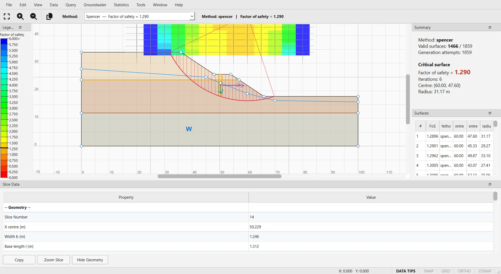
The Interpret window with the factor-of-safety colour grid, the critical circle, the summary and the slice data table — Figure 1.2.6 The Interpret window. The colour of each grid point is the lowest factor of safety of the circles centred there.

A few things worth checking on any analysis:

The minimum is not on the edge of the grid. If the critical centre sits on the border, enlarge the grid and compute again.
The methods agree. Large differences between Bishop and the rigorous methods point at unusual interslice forces (see Section 3.2).
The pore pressures are the ones intended. Query the slices below the water table and check their pore pressure against the head above them.

1.2.8Save and go further#

File → Save writes the model to a .ogr file, plain JSON that the program, the command line, the Python API and the MCP server can all open. From here you can go on to:

Slip surfaces and searchNon-circular surfaces, focus objects and optimisation. Finite-element groundwaterSeepage computed by finite elements instead of a drawn water table; it supplies the pore pressures. Probabilistic and sensitivity analysisRandom strengths and a probability of failure. AI agents and MCPThe same model, built from one sentence.