OGR Slip2D has a single window, the modeller, in which the model is drawn, configured and computed; the results are shown in separate windows. The rest of the user guide follows the menus from left to right.
1.3.1The main window#
The program starts with an empty project called Untitled; the status bar suggests File → Load Demo Slope to start from a small sample model instead. The title bar shows the version and, once the project has been saved or opened, the name of its file.
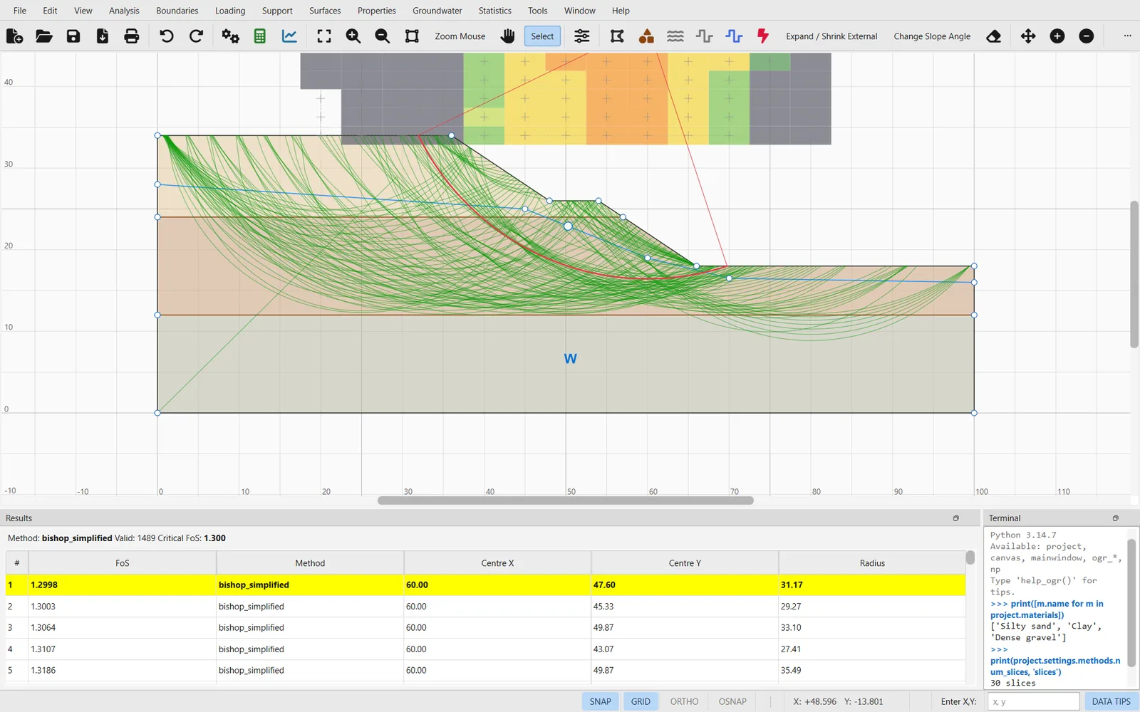
From top to bottom the window holds:
- The menu bar, with the commands of the program (Section 1.3.2).
- The toolbar, with the most used commands as buttons (Section 1.3.3).
- The canvas, where the model is drawn and the results of the last analysis are shown (Section 1.3.4).
- The Results dock, which lists the lowest factors of safety of the last analysis, and the Terminal dock, an embedded Python console, hidden until Window → Terminal is chosen (Section 1.3.6).
- The status bar, with messages on the left and the drawing aids, the cursor coordinates and a coordinate entry field on the right (Section 1.3.5).
1.3.2The menu bar#
The fourteen menus are ordered roughly as a model is built: geometry, loads and supports first, then the slip surfaces, the properties, the groundwater and the statistics.
Commands whose preconditions are not met stay in the menu but are greyed out, and their tooltip says why: Boundaries → Add Water Table once the model has a water table, Boundaries → Add Drawdown Line unless a rapid drawdown analysis is enabled, the grid commands of the Surfaces menu unless the search method uses a grid of centres, and the groundwater and statistics commands until the analysis they belong to is enabled in Project Settings.
Help → Help Topics (F1) shows the address of the source repository; this documentation is the user manual. Help → Check for Updates… shows the installed version and where releases are published; it does not contact any server.
File → Print… only shows a message saying that printing is planned. To print the model view use File → Print Preview…, whose window has its own print button, or export it with File → Export Image…. Edit → Picture Format → Vector (SVG) is recorded but not used: Edit → Copy Image always copies a bitmap of the canvas.
1.3.3The toolbar#
The toolbar is fixed below the menu bar. Its buttons repeat menu commands, in thirteen groups separated by a thin line; hovering over a button shows its name.
| # | Group | Buttons |
|---|---|---|
| 1 | File | New Project, Open Project, Save, Save As, Print |
| 2 | Edit | Undo, Redo |
| 3 | Analysis | Project Settings, Compute, Interpret |
| 4 | View | Zoom All, Zoom In, Zoom Out, Zoom Window, Zoom Mouse, Pan, Select |
| 5 | Display | Display Options |
| 6 | Boundaries | Add External, Material, Water Table, Drawdown Line, Piezometric Line and Tension Crack; Expand / Shrink External; Change Slope Angle; Delete Boundary |
| 7 | Vertices | Move Vertex, Insert Vertex, Delete Vertex |
| 8 | Loading | Add Distributed Load, Add Line Load, Seismic Load, Delete Load |
| 9 | Support | Add Support, Add Support Pattern, Stretch Support, Delete Support |
| 10 | Surfaces | Auto Grid, Add Block Search Window, Surface Options, Define Limits |
| 11 | Properties | Define Materials, Define Support, Assign Materials |
| 12 | Tools | Add Text, Measure, Dimension Length, Dimension Angle, Material Properties Table |
| 13 | Help | Help Topics, About OGR Slip2D |
1.3.4The canvas#
The canvas shows the model section with to the right and upwards, in the length unit of the project (metres unless another unit system is chosen in Section 2.1.2). The cursor position is read out in the status bar.
- Zoom with the mouse wheel, centred on the cursor, or with View → Zoom: Zoom All (F2), Zoom In (F5), Zoom Out (F4), Zoom Window (drag a rectangle) and Zoom Mouse (left click zooms in, right click zooms out).
- Pan by dragging with the middle mouse button at any time, by dragging with Shift held in the Select tool, or with View → Zoom → Pan (F10).
- View → Grid (F7), View → Ruler and View → Grayscale switch the background grid, the rulers and a greyscale rendering.
- View → Display Options… (Ctrl+D) chooses what is drawn: each boundary type, the boundary vertices, the line width, the ruler and grid, support face plates, the finite-element mesh and its numbering, water pressure grid values, flow vectors, ponded water and boundary conditions.
Each boundary type has its own colour, and the water surfaces carry a letter at their midpoint: W on the water table, P on a piezometric line and D on the drawdown line.
Drawing on the canvas#
A drawing command, such as Boundaries → Add External Boundary, puts the canvas in a tool mode, and the status bar says what the tool expects. The conventions are the same for every boundary:
- Click to add a vertex. The point is snapped to vertices, lines and the grid when the drawing aids are on (Snapping).
- Type a vertex instead: write
x, yin the Enter X,Y: field of the status bar and press Enter. Commas, spaces and semicolons are accepted as separators (12.5, 3.2,12.5 3.2,12.5;3.2), with a point as the decimal separator. - Enter finishes the drawing once it has two vertices. The external boundary and the Block Search window are closed polygons and are closed automatically; every other boundary is an open polyline. Clicking again on the first vertex also closes the external boundary.
- Right-click while drawing opens a menu with Done, Close Boundary (external boundary and Block Search window only), Undo last vertex, the Snap, Ortho and OSnap switches, Coordinate Table… (a table of the vertices drawn so far, to correct or extend by typing) and Cancel.
- Esc cancels the drawing in progress and returns to the Select tool.
Picking tools work the same way with a fixed number of clicks: two for a distributed load, a search-grid rectangle, a support (head, then tail) or a support pattern, one for a line load. Some commands ask for typed coordinates in a small dialog instead, as x,y x,y …: the annotation tools of the Tools menu, the focus objects and Add Surface (centre and radius)….
In the Select tool, right-clicking an object opens its context menu. The object under the cursor is chosen in this order: a vertex (Move Vertex, Insert Vertex (after), Edit Coordinates…, Delete Vertex), a load (Modify…, Delete), a support (Properties…, Stretch, Modify Pattern…, Delete), a boundary (Move Boundary, Edit Coordinates…, Convert Boundary…, Delete Boundary, plus a few commands specific to its type) and, on an empty part of a region, a menu to assign a material to that region. Boundaries → Selection Filter… (Ctrl+F) chooses which kinds of object can be picked: boundaries, vertices, materials, supports, loads and slip surfaces, all on by default.
Snapping#
Three drawing aids are switched from the status bar, from the keyboard or from the right-click menu while drawing:
- SNAP (F9, on by default) pulls the cursor onto nearby vertices, onto lines and onto the grid. A circle marks a vertex, a cross a point on a line and a dot a grid node.
- ORTHO (F8, off) locks the segment being drawn to the horizontal or the vertical when it is within a few degrees of either.
- OSNAP (F3, off) draws temporary extension lines from the edges and vertices of nearby boundaries; with SNAP on, the cursor can snap to them.
View → Snap… sets the capture tolerances (in screen pixels, so that they do not depend on the zoom: vertex 12 px, line 10 px, grid node 8 px, extension 8 px), the angular window of ORTHO (5°) and the data-tip mode, and has a Restore Defaults button. The snapping grid follows the zoom: its spacing is a round number (1, 2 or 5 times a power of ten) about 60 pixels wide on screen.
The Grid spacing fields of the Snap dialog have no lasting effect: the canvas replaces them with the zoom-dependent spacing as soon as the cursor moves. The shortcut Ctrl+Shift+S is assigned both to View → Snap… and to File → Save As…; use the menus for either.
Undo and redo#
Edit → Undo (Ctrl+Z) and Edit → Redo (Ctrl+Y) step through the edits of the geometry (adding, deleting, moving, converting and reshaping boundaries and their vertices) and the painting of materials onto regions with Properties → Assign Materials. Edits made in dialogs (materials, loads, supports, settings) are not on the undo stack; while the dialog is open, the only way back is Cancel. The stack is cleared when a project is created, opened or replaced by the demo slope.
1.3.5The status bar#
The left part of the status bar shows messages: what the active tool expects, what the last command did, and the factor of safety of the last analysis. A message stays for a few seconds and is replaced by the next one; the complete list of notes of an analysis is in Analysis → Analysis Notes… (Section 1.3.6). The right part holds the permanent indicators.
| Indicator | Meaning | Key | At start |
|---|---|---|---|
| SNAP | Snap to vertices, lines and grid nodes | F9 | on |
| GRID | Show the background grid (the same switch as View → Grid) | F7 | on |
| ORTHO | Horizontal and vertical segments only | F8 | off |
| OSNAP | Extension lines from nearby boundaries | F3 | off |
| X, Y | Cursor coordinates, to three decimals | — | — |
| Enter X,Y: | Typed vertex for the drawing in progress (Drawing on the canvas) | Enter | — |
| DATA TIPS | Property tips under the cursor (Data tips) | — | on |
Data tips#
With DATA TIPS on, hovering over a material region, a support or a load in the Select tool shows its properties, with their units, in a tooltip. The View → Snap… dialog offers three levels: None, Minimum (only the identity: the name of the material, the type of the support, the magnitude of the load) and Maximum (every property, the default). The status-bar switch alternates between Maximum and None.
1.3.6Docks and panels#
Results dock. After Analysis → Compute (Ctrl+T) the dock along the bottom shows, for the first of the enabled methods, the number of valid surfaces and the critical factor of safety, followed by a table of the 50 surfaces with the lowest factor: rank, factor of safety, method, centre , centre and radius. The critical surface is the first row, highlighted. With a design standard switched on, the caption reads Over-design factor instead of Critical FoS (Section 2.11). The results of the other methods are in the Interpret window.
The docks can be moved, floated and closed. A closed dock is brought back by right-clicking the toolbar, which lists the toolbar and the docks with a tick each.
Selecting a row of the Results dock does not yet highlight its surface on the canvas; use Analysis → Interpret to inspect individual surfaces.
Terminal dock. Window → Terminal (Ctrl+`) opens an embedded Python console that runs inside the program, with the live model as project, the canvas as canvas, the window as mainwindow, NumPy as np and the packages ogr_core and ogr_slip2d; help_ogr() prints a few examples. Enter runs the input, Shift+Enter starts a new line, Ctrl+↑ and Ctrl+↓ move through the history and Ctrl+L clears the console. Code typed there can change anything in the model; scripting is described in Section 2.12.
Analysis notes. An analysis can produce several notes: a method that could not run, a setting the chosen search does not read, a design standard that turns the result into an over-design factor. The status bar shows the first one followed by [+n more — Analysis > Analysis Notes]; Analysis → Analysis Notes… opens a panel with all of them, the notes of the last statistical run included.
Info Viewer. Analysis → Info Viewer (Ctrl+I) summarises the model: number of boundaries, materials, supports and loads, the bounding box, the search method and the author.
Assign Materials panel. Properties → Assign Materials opens a floating panel with the list of materials; see Section 2.3.3.
1.3.7The Interpret window#
Analysis → Interpret opens the results of the last analysis in a separate window titled OGR Slip2D — Interpret — followed by the project name. Its canvas is read-only, so the model cannot be changed from it; several Interpret windows can be open at once, and each one keeps the results it was opened with. File → Close (Ctrl+W) closes it.
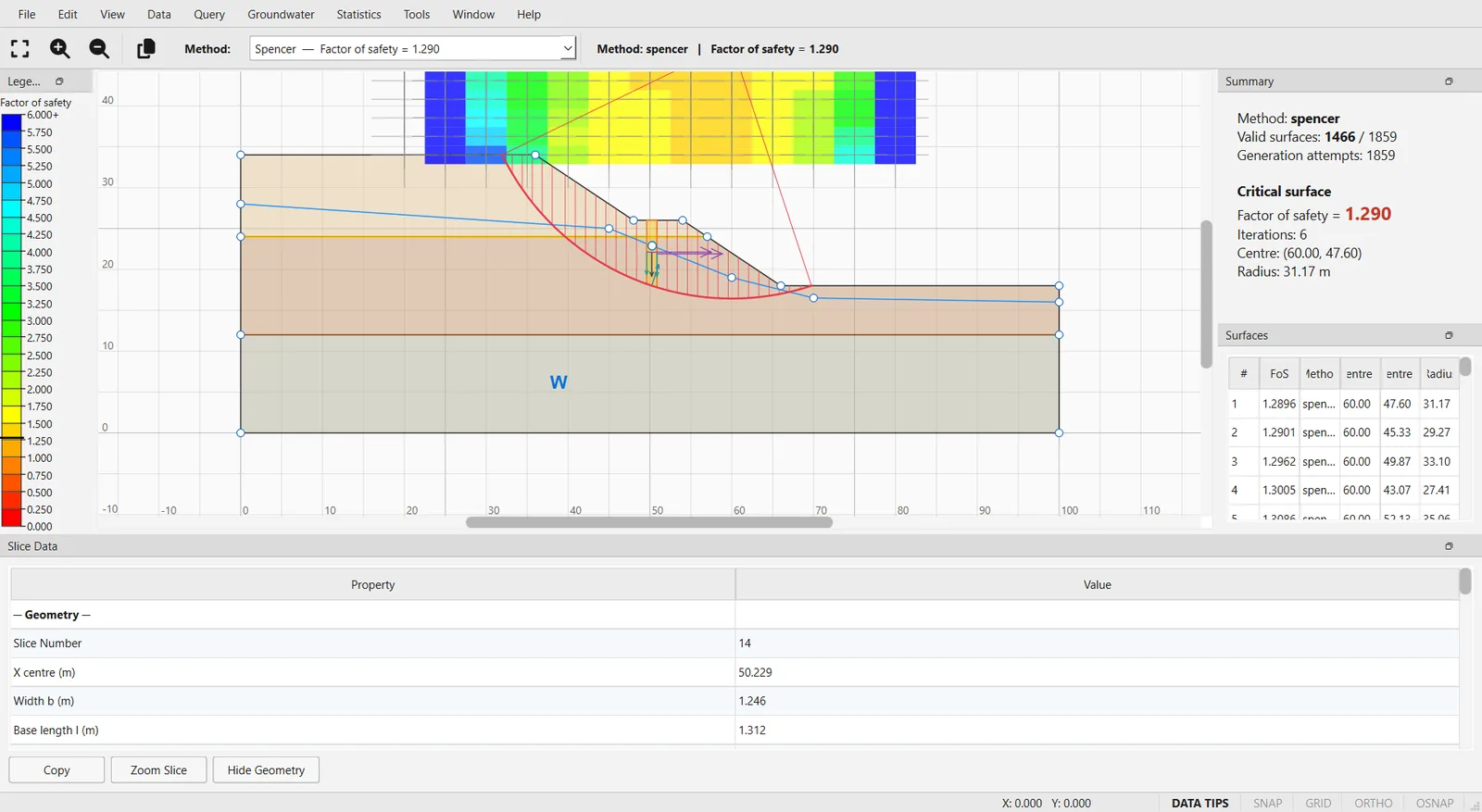
- Docks: the colour Legend on the left; Summary and Surfaces (the 100 surfaces with the lowest factor of safety) on the right; Slice Data at the bottom. Window shows or hides the last three and View → Show Legend the first.
- Method selector: when several methods were computed, a drop-down list at the top switches the whole window between them.
- Hover preview: with a grid search, hovering over a centre of the grid draws the lowest surface of that centre and gives its factor of safety in the status bar.
Its menus are File (export the image or the surface data as CSV), Edit, View (zoom, legend, contour and legend options), Data (which surfaces are drawn: global minimum, minimum per centre or all; filters; the factor of safety along the slope; data exports; invalid surfaces; support forces and back analysis), Query (queries, slices, line of thrust, values along the surface, free-body diagram of a slice, surfaces through a point, result table), Groundwater, Statistics (histogram, cumulative, scatter, sensitivity and convergence plots), Tools, Window and Help. Commands that need something the project does not have (a transient analysis, supports, statistical results) are greyed out, with a tooltip saying what is missing. The window is described in Section 2.8.
A few commands of the Interpret window do nothing yet: View → Data Tips, the four display switches at the top of the Groundwater menu (Phreatic Surface, Piezometric Lines, Flow Vectors, Streamlines) and Tools → Measure and Tools → Dimension Length.
1.3.8Other result windows#
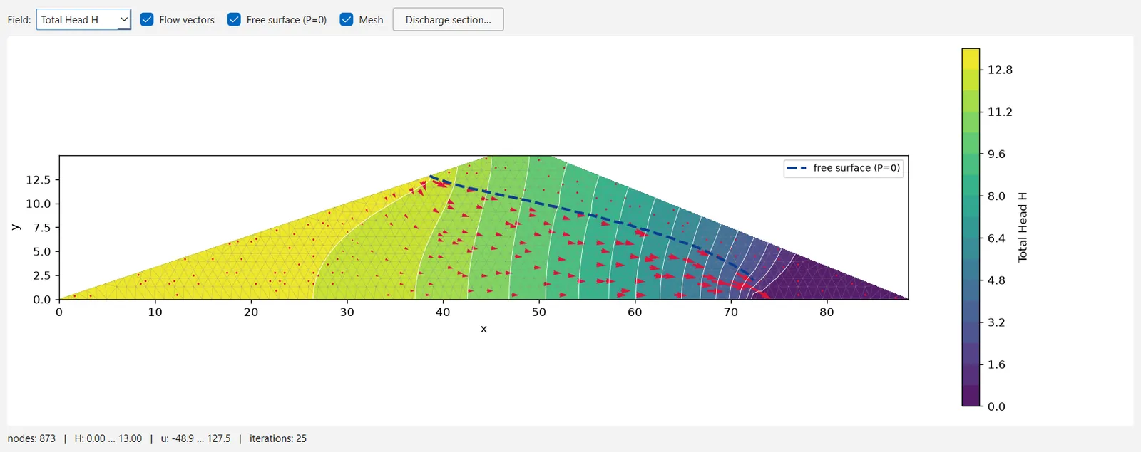
Interpret Groundwater (Groundwater → Interpret Groundwater, available once a finite-element seepage analysis has been computed) shows the seepage field over the mesh: total head , pressure head or pore pressure , with switches for the flow vectors, the free surface () and the mesh, a Discharge section… tool for the flow through a section and, for a transient analysis, a stage selector and a plot of the factor of safety against time. See Section 2.9.
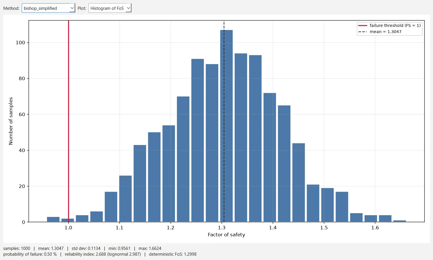
Statistics (Statistics → Show Statistics, opened automatically after Statistics → Compute Statistics) presents a probabilistic or sensitivity run: the histogram of the factor of safety with the probability of failure and the reliability index, the convergence of the mean and of the probability of failure with the number of samples, scatter plots against each random variable and the sensitivity plot. See Section 2.10.
Groundwater → Drawdown Level Sweep… ends with a chart of the factor of safety against the drawdown level, and Data → Support Force Diagram… in the Interpret window opens the force diagram of a support. These charts open in windows of their own.
Several projects at once#
Window → New Window opens a second, independent modeller with its own project. The Window menu lists the open windows, marks the active one with a bullet and those with unsaved changes with an asterisk, and brings any of them to the front; Window → Close Window closes the current one.
Annotations#
The Tools menu draws on a separate annotation layer that the analysis never reads: lines, arrows, polylines, polygons, rectangles, circles and text (Tools → Draw), length, angle and horizontal or vertical dimensions (Tools → Dimensions, and Tools → Measure), axes and a background image. Points are typed as coordinates. Tools → Annotations manages, shows, hides and deletes them. Tools → Convert Tool to Boundary… is the only way an annotation becomes model geometry: it copies a line, polyline, polygon, rectangle or circle into an external boundary, a material boundary, a water table, a piezometric line or a tension crack, and keeps the annotation. Tools → Property Tables shows read-only tables of the materials, the supports and the hydraulic properties, with a button to copy them to the clipboard.
1.3.9Preferences#
File → Preferences… sets the language (English or Español) and the theme (Light or Dark) and applies them with Save.
- The theme changes at once.
- The language applies to the dialogs and windows opened afterwards (including a window opened with Window → New Window); the menus of the windows already open keep their language.
- Neither choice is stored: the program always starts in English with the light theme.
Menu names in this documentation are those of the English interface.
The three check boxes in the lower group of the Preferences dialog (Show Tabs for Multiple Windows, Mark file as modified after importing and Default to compressed format when saving) are not connected to anything yet.
1.3.10The agent bridge#
An AI agent connected through the MCP server can work on the model open in the window, where every edit is seen as it happens. Tools → Agent bridge (MCP) controls this connection. It is switched on when the program starts, unless the program is started with ogr-slip2d --no-agent-bridge, and the status bar then gives the process number and port: Agent bridge on (pid …, port …).
- The bridge listens only on the local machine (
127.0.0.1) and requires a random token; the agent's server finds it when started withogr-slip2d-mcp --attach. - An edit made by the agent is one step of Edit → Undo, and an analysis it runs is shown in the Results dock and on the canvas, as a Compute would be.
- While the window is computing, the agent's edits are refused, so that the model does not change under the analysis.
- Unticking the menu entry closes the bridge.
Setting up an agent is described on the AI & MCP page and the tools it can use in Section 5.1.
1.3.11Keyboard shortcuts#
| Keys | Command |
|---|---|
| Ctrl+N | File → New Project |
| Ctrl+O | File → Open Project… |
| Ctrl+S | File → Save |
| Ctrl+Shift+S | Assigned to both File → Save As… and View → Snap… (see Snapping) |
| Ctrl+P | File → Print… |
| Ctrl+Q | File → Exit |
| Ctrl+Z / Ctrl+Y | Edit → Undo / Edit → Redo |
| F2, F5, F4 | Zoom All, Zoom In, Zoom Out |
| F10 | View → Zoom → Pan |
| Esc | Cancel the drawing in progress and return to Select |
| F7 | View → Grid |
| F9, F8, F3 | SNAP, ORTHO, OSNAP on or off |
| Ctrl+D | View → Display Options… |
| Ctrl+J | Analysis → Project Settings… |
| Ctrl+I | Analysis → Info Viewer |
| Ctrl+T | Analysis → Compute |
| Ctrl+1 … Ctrl+8 | Boundaries → Add External Boundary, Add Material Boundary, Add Water Table, Add Drawdown Line, Add Piezometric Line, Add Tension Crack, Add Weak Layer, Add Anisotropic Surface |
| Ctrl+F | Boundaries → Selection Filter… |
| Ctrl+` | Window → Terminal |
| F1 | Help → Help Topics |
| Enter | Finish the drawing in progress; in the Enter X,Y: field, add the typed vertex |
| Ctrl+W | File → Close, in the Interpret window |