Instead of drawing a water table, OGR Slip2D can compute the pore pressures of the slope by a finite-element seepage analysis, steady or in stages through time, and hand them to the limit-equilibrium analysis. The Groundwater menu is ordered as the workflow, and each command becomes available only when the step before it has been done. The equations are in Section 3.7.
2.9.1The workflow#
| Step | Command | Available when |
|---|---|---|
| 1 | Analysis → Project Settings → Groundwater: Method fea_steady or fea_transient | always |
| 2 | Properties → Define Materials…: Water Parameters, Type fem, for every material that takes the field (Section 2.9.8) | always; see the note there |
| 3 | Groundwater → Define Hydraulic Properties… | the method is a finite-element one and materials exist |
| 4 | Groundwater → Mesh → Generate FE Mesh… | always (needs an External Boundary) |
| 5 | Groundwater → Set Boundary Conditions… | a mesh exists |
| 6 | Groundwater → Transient Groundwater… (only for a staged analysis) | the method is a finite-element one |
| 7 | Groundwater → Compute Groundwater | a mesh exists |
| 8 | Groundwater → Interpret Groundwater | a groundwater result exists |
| 9 | Analysis → Compute | — |
2.9.2Choosing a finite-element method#
In Analysis → Project Settings → Groundwater, set Method to fea_steady or fea_transient. The program treats the two in the same way: whether the analysis runs in stages is decided by the Advanced group of the same page, where Transient groundwater is one of four mutually exclusive choices (with None, Calculate Excess Pore Pressure (B-bar method) and Rapid Drawdown analysis). With a finite-element method:
- the hydraulic commands of the Groundwater menu become available;
- Properties → Define Materials… shows two unsaturated-strength fields for each material, Unsaturated Shear Strength Angle (φb) and Air Entry Value, both 0 by default, so that suction adds no strength unless you ask for it (Section 3.6). Negative pore pressure cutoff on the Groundwater page caps the suction they can use;
- a reservoir is not drawn: it is the total head you prescribe on the boundary, and the stability analysis applies the weight of the standing water wherever that head is above the ground. Do not draw a water table on top of it.
2.9.3Hydraulic properties#
Groundwater → Define Hydraulic Properties… lists the materials on the left (names and colours are edited in Define Materials) and the permeability of the selected one on the right. A material you never edit here keeps the defaults: constant permeability with Ks = 1 × 10⁻⁶.
| Field | Meaning | Default |
|---|---|---|
| Saturated permeability Ks | Permeability K1 of the saturated soil. Disabled for User Defined, which takes it from the first point of its curve. | 1 × 10⁻⁶ |
| K2 / K1 | Anisotropy: ratio of the second principal permeability to the first. | 1 |
| K1 angle (deg from +X) | Direction of K1. | 0° |
| Model | How the permeability falls in the unsaturated zone: Constant, Simple (with a soil type: General, Sand, Silt, Clay or Loam), Brooks-Corey, Fredlund-Xing, Gardner, van Genuchten or User Defined. The parameters of the chosen model appear below it. | Constant |
Pick… loads representative literature parameters for Brooks-Corey, Fredlund-Xing, Gardner and van Genuchten; Plot… draws the permeability against suction for the material shown.
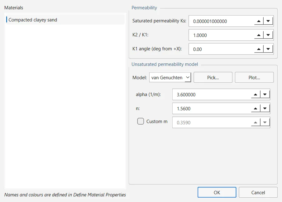
The program converts neither Ks nor the stage times: Permeability Units and Time Units on the General page of Project Settings only label them, and the dialog shows no unit. A steady analysis does not depend on the unit as long as every material uses the same one, but a transient analysis does: give the stage times in the time unit of Ks (seconds for Ks in m/s). Note that the two labels default to m/s and days.
2.9.4The finite-element mesh#
Groundwater → Mesh → Generate FE Mesh… asks for the approximate number of elements (1000 by default; 20 to 200 000) and meshes every material region of the model with three-node triangles, the nodes shared along the contacts, so each element takes the material the limit-equilibrium analysis reads for that region. The status bar reports the number of elements and nodes and the smallest angle of the mesh.
Boundary conditions are attached to node numbers, so a new mesh (or Groundwater → Mesh → Reset FE Mesh) drops the boundary conditions, the computed field, the transient results and the conditions stored with the transient stages, and says so in the status bar. The stages themselves keep their times, labels and flags.
2.9.5Boundary conditions#
A mesh starts with default conditions: Unknown (P=0 or Q=0) on the ground surface, slope face included, and zero nodal flow on the left, right and bottom edges. These prescribe no head anywhere, and a steady problem without a prescribed head has no solution, so at least one head must be set before computing.
Groundwater → Set Boundary Conditions… assigns a condition to a whole side of the model at a time. Choose the Type, enter the Value where the type takes one, select the target in Apply to (Left edge, Right edge, Bottom edge or Ground surface, each with its number of nodes) and press Assign. Restore defaults goes back to the default conditions. The summary line counts the nodes of each type.
| Type | Value | Seepage face |
|---|---|---|
| Total Head | head H (m) | — |
| Pressure Head | head P (m) | — |
| Zero Pressure | — | — |
| Nodal Flow Rate | flow at each node | allowed |
| Infiltration | flux on the boundary segments; applied to segments only | allowed |
| Unknown (P=0 or Q=0) | — | decided by the solver, node by node: P = 0 where water seeps out, Q = 0 elsewhere |
Two more targets at the bottom of the list prescribe a reservoir: Reservoir on the left, at Value and Reservoir on the right, at Value. Enter the water level as the Value and press Assign: every boundary node the water reaches (the vertical edge on that side and the ground surface inwards for as long as it stays at or below the level) receives a total head equal to the level, and the dialog reports how many nodes were submerged. A reservoir that reaches only a node or two is usually a level typed below the toe.
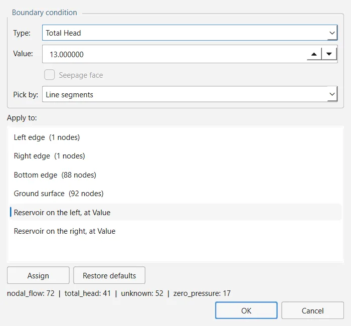
In version 0.1.235 the Pick by selector of the dialog (Line segments or Nodes) has no effect: a condition always goes to every node of the chosen side, and infiltration to its segments. OK keeps the conditions; Cancel discards everything assigned since the dialog opened.
2.9.6Computing the field#
Groundwater → Compute Groundwater solves the steady field, or the stages of a transient analysis when one is configured. A steady solve reports the number of iterations and the range of pore pressure in the status bar, and names any material that used the default hydraulic properties; when it does not converge, the status bar says why. The field is saved in the .ogr file, so reopening a project does not require computing it again.
The steady analysis solves for the total head on linear triangles, with the permeability reduced in the unsaturated zone by the model of each material, by under-relaxed Picard iteration (relaxation 0.4, at most 200 iterations, tolerance 10⁻⁵ m). Nodes of type Unknown switch between seepage face and no-flow until they settle (Neuman, 1973). The transient analysis solves Richards' equation in mixed form with implicit time steps (Celia, Bouloutas & Zarba, 1990).
Source: ogr_slip2d/transient_stability.py · ogr_fem2d/solvers/2.9.7Interpreting the field#
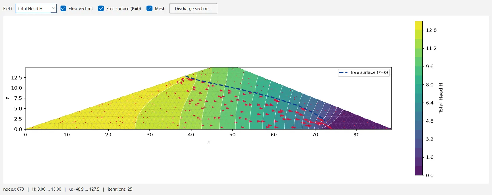
Groundwater → Interpret Groundwater opens the Interpret Groundwater window. Its bar offers:
- Field: filled contours of Total Head H, Pressure Head P or Pore Pressure u, suction showing as negative values;
- Flow vectors (on): the Darcy velocity of the elements;
- Free surface (P=0) (on): the line of zero pressure;
- Mesh (off): the element edges;
- Discharge section…: asks for a section as
x0,y0,x1,y1and reports the flow through it per unit width, positive towards the normal of the section (the direction from the first point to the second turned 90° anticlockwise); - for a transient run, a Stage list, with [SF] on the stages that computed a factor of safety, and FoS vs time….
The line below the plot gives the number of nodes, the ranges of head and pore pressure, the iterations, the seepage-face nodes and, for a stage, its time and factors of safety; NOT CONVERGED appears when the solve did not converge.
The groundwater fields can also be contoured over the stability results, in the Interpret window of Analysis → Interpret, with View → Contour Options…; its Groundwater menu adds the iteration history, a convergence plot, a query of head at a point and Export All Nodal Values… to CSV (Section 2.8).
2.9.8Using the field in the stability analysis#
The computed field reaches the limit-equilibrium analysis only through the materials whose Water Parameters → Type is fem: at the base of every slice of such a material, the pore pressure is interpolated from the nodal values of the element that contains it. A slice base outside the mesh gets no pore pressure. A material left on any other type ignores the field entirely.
In version 0.1.235 Define Materials hides the whole Water Parameters group while the groundwater method is fea_steady or fea_transient, so the Type cannot be changed then. Set Type to fem for the materials concerned before choosing the finite-element method, or switch the method back for a moment to change it. The same coupling can be set through the MCP server or the Python API (Section 5.1).
Compute refuses to run while a material of type fem has no computed field to read, rather than report the pore pressure as zero, which would look like a dry slope. Generating a new mesh clears the field, so compute the groundwater again after remeshing. After a transient analysis the field stored in the project is that of the last stage.
2.9.9Transient analysis#
A staged analysis is set up in Groundwater → Transient Groundwater…. Its first box does the same as choosing Transient groundwater in the Advanced group of Analysis → Project Settings → Groundwater.
- Transient groundwater analysis switches the staged analysis on or off; switching it on turns off the other advanced option, if one was chosen.
- Stages: a table with Time, Calculate SF and Label. Add stage adds a row at twice the latest time (1 for the first), Delete stage removes the selected rows. Times must be positive and distinct; the stages are sorted by time.
- Capture current BCs stores the conditions currently set in Set Boundary Conditions in the selected stage, which is marked [BC]. A stage without conditions of its own uses the current ones, and the field only evolves where a stage's conditions differ from the initial ones.
- Capture as initial state stores the current conditions as the initial state: the steady field the run starts from. Without it, the current conditions are used, so the model starts in equilibrium with them.
- Transient FEA options: Tolerance (1 × 10⁻⁵), Maximum iterations (30) and Number of time steps per stage (Auto by default: derived from the element size and the storage, so that the water front crosses about one element per step). The same three are on the Transient page of Project Settings, which is greyed out unless the transient option is on.
For a drawdown, for example, assign a reservoir at the initial level and capture it as the initial state. Then press Restore defaults in Set Boundary Conditions (assigning a lower reservoir does not clear the heads of the nodes it no longer reaches), assign the reservoir at the lower level, and any other condition again, select a stage and capture it. Compute Groundwater solves the stages in order and computes the factor of safety, with every enabled method, at the stages marked Calculate SF. They are plotted against time by FoS vs time… in Interpret Groundwater and by Data → Graph SF with Time… in the Interpret window. If no material is of type fem, the run warns that the stage factors would ignore the computed pressures.
The transient analysis also uses the saturated and residual water contents (0.4 and 0.05) and the specific storage (1 × 10⁻⁵ 1/m) of each material. Define Hydraulic Properties does not show them in version 0.1.235; they keep these defaults unless they are set through the MCP server or the Python API.
2.9.10Drawdown Level Sweep#
Groundwater → Drawdown Level Sweep… belongs to the limit-equilibrium rapid-drawdown analysis, not to the finite-element one: it needs Rapid Drawdown analysis selected in the Advanced group, a groundwater method based on water surfaces, and at least one material with undrained behaviour (Section 2.4, Section 3.8). The sweep is needed because the critical reservoir level is not always the lowest one.
The dialog asks for the Number of levels (11 by default; 2 to 101), spaced evenly from the initial water table down to the lowest ground of the model, and whether to Include total drawdown (ticked). Each level is a full search with every enabled method, so the cost of the run grows with the number of levels. The status bar then gives the critical level and its factor of safety (and, when the total drawdown would overstate it, by how much), and a chart plots the factor of safety against the drawdown level.