Probabilistic and sensitivity analysis — OGR Slip2D documentation

A probabilistic analysis treats some inputs of the model as random variables, draws samples of them and recomputes the factor of safety for each sample, which gives its distribution, the probability of failure and the reliability index. A sensitivity analysis instead sweeps one input at a time across its range. Both are set up in Project Settings and in the Statistics menu, and their output is read in the Statistics window; the statistics behind them are in Section 3.11.

Version 0.1.235

In this version the run cannot be completed from the window's menu: see Section 2.10.4. The settings below are still the ones the analysis uses when it is run through the MCP server or the Python API.

2.10.1Enabling the analysis#

Both analyses are switched on in Analysis → Project Settings → Statistics. Until one of them is ticked, the commands of the Statistics menu stay greyed out: Random Variables… becomes available first, Compute Statistics once at least one random variable is defined, and Show Statistics once there are results to show.

Table 2.10.1 The Statistics page of Project Settings.

Field	What it does	Default
Probabilistic analysis	Samples the random variables and recomputes the factor of safety for each sample.	off
Sensitivity analysis	Sweeps each random variable across its range, one at a time.	off
Analysis type	Global Minimum evaluates every sample on the critical surface of the deterministic analysis. Overall Slope repeats the whole search for every sample, so the location of the critical surface is not assumed fixed; it is much slower.	Global Minimum
Sampling method	Monte Carlo or Latin Hypercube.	Monte Carlo
Number of samples	N (1 to 1 000 000).	1000
Sensitivity intervals	Equal intervals into which each variable's range is divided for the sensitivity sweep (2 to 500); intervals + 1 values are evaluated.	50

2.10.2Random variables#

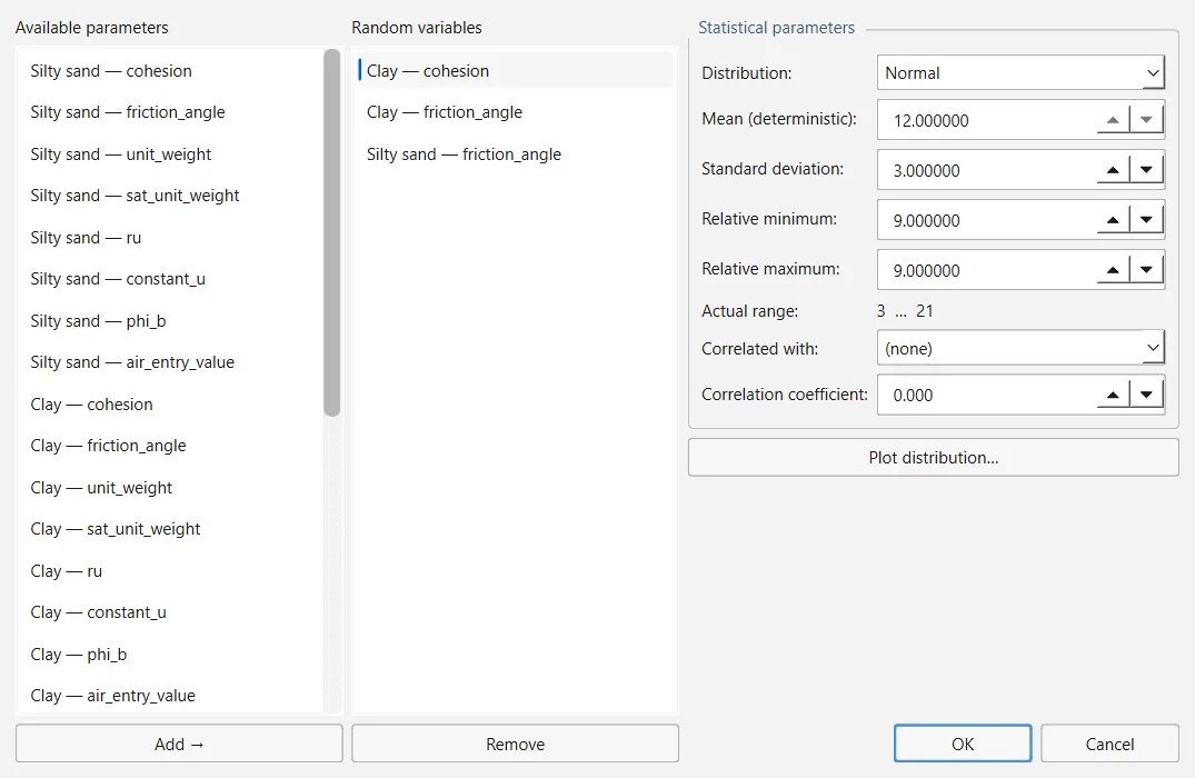
Statistics → Random Variables… opens a dialog in three columns. Available parameters lists every input of the model that can become random; select one and press Add → to move it to Random variables (Remove takes it back). The selected variable's distribution is edited on the right. The parameters on offer are:

the parameters of each material's strength model (cohesion, friction angle and the parameters of the other models);
each material's unit weight and saturated unit weight, r_u, constant pore pressure, unsaturated shear strength angle φ^b and air entry value;
the hydraulic parameters of each material that has them;
the parameters of each support;
the magnitudes of the distributed and line loads;
the seismic coefficients k_h and k_v;
a vertical offset of the water table, when the model has one.

Table 2.10.2 Statistical parameters of a random variable.

Field	What it does
Distribution	Normal, Uniform, Triangular, Beta, Exponential, Lognormal or Gamma.
Mean (deterministic)	The value in the model; read-only. To change the mean, change the model.
Standard deviation	Used by Normal, Lognormal, Beta and Gamma; greyed out for the others.
Relative minimum, Relative maximum	How far below and above the mean the variable may go. Actual range shows the result, from mean − relative minimum to mean + relative maximum.
Correlated with, Correlation coefficient	Another random variable of the model and a coefficient between −1 and 1. A negative coefficient between cohesion and friction angle is the usual case.

A variable just added is Normal, with a standard deviation of 10 % of its mean and relative limits of 30 % of the mean on each side (0.1 and 0.3 when the mean is zero, as for a seismic coefficient or the water-table offset). Plot distribution… draws the probability density that will be sampled, with the mean marked.

The Random Variables dialog: available parameters on the left, the random variables in the middle and the distribution, standard deviation, relative limits and correlation of the selected variable on the right — Figure 2.10.1 Statistics → Random Variables.

In OGR Slip2D

Distributions are truncated to their actual range: samples are drawn by inverting the distribution between the two limits, so no value falls outside them and Latin Hypercube strata survive the truncation. A declared correlation is imposed by reordering the ranks of the second variable, which leaves both marginal distributions unchanged (Iman & Conover, 1982). Each sample is applied to a copy of the model, so the run does not modify your project.

Source: ogr_core/statistics/distributions.py · ogr_core/statistics/random_variables.py

2.10.3Sampling and the seed#

Monte Carlo draws every sample independently. Latin Hypercube divides the probability range of each variable into N strata and draws one sample in each, which usually needs fewer samples for the same accuracy (McKay, Beckman & Conover, 1979).

The random numbers are set in Analysis → Project Settings → Random Numbers:

Generation: Pseudo-random (default) is reproducible: the same Seed (10116 by default) gives the same samples, and therefore the same answer, every time; Random takes the seed from the clock, so successive runs differ, which is a way to check that a conclusion is not an artefact of one seed. The Seed box is greyed out under Random.
Share one Latin Hypercube stratification across variables (off): sample i then sits in the same stratum of every variable, so all of them are unfavourable together. It answers a different question from the independent case and usually widens the spread. It does nothing under Monte Carlo.

The same page also seeds the random slip-surface searches (Section 2.7).

2.10.4Computing the statistics#

Statistics → Compute Statistics first runs the deterministic analysis, with every enabled method and its search, to find the critical surface of each method. Then:

a Global Minimum analysis evaluates the N samples on the critical surface of each method (each method keeps its own);
an Overall Slope analysis repeats the whole search N times. Besides the distribution of the minimum factor of safety, it records the critical surface of every sample and the critical probabilistic surface: the individual surface with the highest probability of failure among those evaluated at least five times, which need not be the deterministic critical surface;
a sensitivity analysis is computed as described below.

With a design standard active, every sample is factored like the deterministic model, so the statistics describe the over-design factor (Section 2.11). With a seismic analysis mode on (critical seismic coefficient or Newmark displacement), the statistics are taken on the factor of safety of the surface with the lowest critical seismic coefficient, which is not necessarily the lowest factor of safety of the sample; the analysis notes say so.

Compute Statistics fails from the menu in version 0.1.235

Started from the window, the run stops with an internal error (TypeError: cannot pickle 'MainWindow' object) when it tries to copy the model for the first sample, after the deterministic analysis. The window shows no message, no statistics are produced and Show Statistics stays greyed out. The same analysis runs through the MCP server (its statistics_run tool) and through the operations of the Python API, which copy the model in a way that works (Section 5.1, Section 5.3).

2.10.5The Statistics window#

After a successful run the Statistics window opens by itself; Statistics → Show Statistics opens it again. Choose the Method and the Plot:

Histogram of FoS: the factors of safety of the samples, with the failure threshold (F = 1) and the mean marked. The line below gives the number of samples, mean, standard deviation, minimum and maximum, the probability of failure, the reliability index (normal and lognormal) and the deterministic factor of safety.
Convergence: the mean factor of safety and the probability of failure against the number of samples. A flat tail means the sample count is sufficient; a curve still drifting means more samples are needed.
Sensitivity: the factor of safety against each variable, as a percentage of its range, with the variables ranked by how much they move it.

When a run could not sample every variable (for example, because a variable refers to a material that has since been deleted), the window says so in red above the plot.

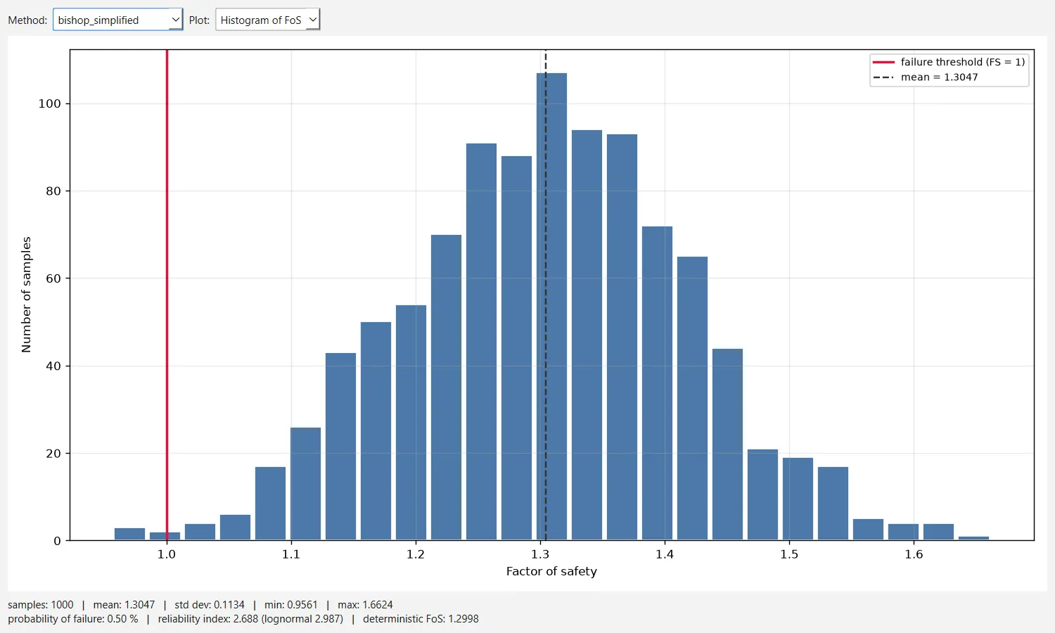
The Statistics window showing the histogram of the sampled factors of safety with the failure threshold and the mean marked, and the summary statistics below — Figure 2.10.2 The Statistics window with the histogram of the factor of safety.

The probability of failure and the reliability indices are computed from the N valid samples:

P_f = \dfrac{n(F < 1)}{N}

\beta = \dfrac{\mu_F - 1}{\sigma_F} \qquad \beta_{\mathrm{LN}} = \dfrac{\mu_{\ln F}}{\sigma_{\ln F}}

where

$n(F < 1)$: number of samples with a factor of safety below 1
$\mu_F,\ \sigma_F$: mean and standard deviation of the factors of safety
$\mu_{\ln F},\ \sigma_{\ln F}$: mean and standard deviation of their natural logarithms, for the lognormal index

2.10.6The Statistics menu of the Interpret window#

The Interpret window (Section 2.8) has its own Statistics menu. Its first three plots do not use the probabilistic samples: they are drawn from the factors of safety of the surfaces analysed by the search, and are available after any Compute.

Table 2.10.3 The Statistics menu of the Interpret window.

Command	What it shows	Needs
Histogram Plot…	Histogram of the factors of safety of the valid surfaces of the search (25 bins, adjustable).	a Compute
Cumulative Plot…	Cumulative distribution of the same factors of safety.	a Compute
Scatter Plot…	Factor of safety against radius, for the valid surfaces of the search.	a Compute
Sensitivity Plot…	The sensitivity curves of the first method.	statistics results
Convergence Plot…	Mean factor of safety and probability of failure against the number of samples.	statistics results
Export Statistics Data…	A CSV file with one row per sample: its number, the value of every random variable and the factor of safety.	statistics results
Show GM Surfaces, Pick GM Surfaces	Draws, or lists for selection, every minimum the result reports: the critical surface of each sample of an Overall Slope run, or the regions a Particle Swarm Search with several minima told apart.	either of those
Critical Probabilistic Surface	Gives the probability of failure and the reliability index of the critical probabilistic surface in the status bar.	an Overall Slope run

Commands that need statistics results are greyed out until there are some, with a tooltip saying so. Show GM Surfaces and Pick GM Surfaces do not need them: they also work after a Particle Swarm Search with Report several minima ticked, which in version 0.1.235 is the only way to use them from the window.

2.10.7Sensitivity analysis#

For each random variable in turn, the sensitivity analysis divides its actual range into the number of Sensitivity intervals (50 by default, so 51 values) and recomputes the factor of safety on the critical surface of each method at every value, with all the other variables held at their means. Only the minimum and maximum of each variable are used: the distribution, the standard deviation and the correlations play no part, and no probability of failure comes out of it. Its result shows which inputs matter most, and how far one of them can move before the factor of safety reaches 1.

2.10.8Reading the results#

Check the convergence plot before quoting a probability of failure: if the value still changes as samples are added, more samples are needed.
A Global Minimum run assumes that the critical surface does not move with the samples. When the inputs could change the mechanism (a weak layer whose strength varies, for instance), compare with an Overall Slope run.
The reliability index assumes a normal or lognormal distribution of the factor of safety. The probability of failure is the fraction of samples with $F < 1$ and assumes no distribution, so with few samples a small probability is poorly resolved.
A sample that cannot be evaluated is left out, and the run reports how many were.