Each region of the model is made of one material, which sets its unit weight, its strength and the source of its pore pressure. Materials are defined in one dialog and then painted onto the regions of the model.
2.3.1Defining materials#
Open Properties → Define Materials… (also on the toolbar, and in the right-click menu of a region). The list on the left holds the materials of the project, each in its colour; + Add creates one and − Remove deletes the selected one. A new material is called Material n and starts as Mohr–Coulomb with kPa and .
The editor on the right shows the selected material in up to five groups: General and Strength Type always, Water Parameters unless the project uses a finite-element groundwater method, and Rapid Drawdown Parameters and Excess Pore Pressure only when the project runs those analyses. Edits are kept while you move from one material to another; OK stores the whole list and Cancel discards every change made since the dialog was opened. There is no Apply button.
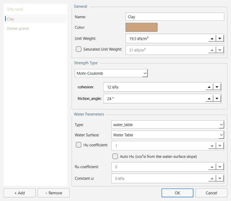
General#
| Field | Meaning | Default |
|---|---|---|
| Name | Name of the material, as listed and reported | Material n |
| Color | Colour of its regions on the canvas; the button opens a colour picker | light brown |
| Unit Weight | Bulk unit weight | 20 kN/m³ |
| Saturated Unit Weight | Optional saturated bulk unit weight, used below the water table. Available only when the model has a water table. | off / 21 kN/m³ |
| Unsaturated Shear Strength Angle | , the angle that adds strength for matric suction; 0 means suction adds nothing. Shown only with a finite-element groundwater method. | 0° |
| Air Entry Value | Suction below which the saturated friction angle still governs. Shown only with a finite-element groundwater method. | 0 kPa |
The saturated unit weight is the bulk unit weight of the saturated soil, not the submerged (buoyant) one, so it should be greater than the unit weight above the water table; the dialog shows a warning in red when it is not, and keeps the value as typed. The two unsaturated parameters follow the extended Mohr–Coulomb envelope of Fredlund, Morgenstern & Widger (1978); they only matter where a seepage analysis gives negative pore pressures (Section 3.6).
Strength type#
The drop-down list of the Strength Type group offers 22 strength models. The equation of the chosen model is shown beside the list, and its parameters appear below it, each labelled with the name under which it is stored and with a tooltip that describes it. Models defined by a table (the shear/normal, discrete, C/Phi and anisotropic functions and the ranges of Generalized Anisotropic) show the table instead, with + Row and − Row buttons. Snowden Modified Anisotropic Linear has two buttons, Bedding Strength Function… and Rock Mass Strength Function…, and the depth-dependent undrained models an Apply cutoff box.
| Strength type | Parameters (starting values) |
|---|---|
| Mohr-Coulomb | cohesion 10, friction_angle 30 |
| Undrained (φ=0) | cohesion 50, the undrained strength |
| Infinite Strength | none; the slip surface cannot pass through it |
| No Strength (water) | none; for water or material with no shear strength |
| Generalized Hoek-Brown | sigci 50 000, mb 2.5, s 0.004, a 0.5; GSI… derives mb, s and a (Section 2.3.2) |
| Hoek-Brown | sigci 15 000, m 0.357, s 0.0017 |
| Power Curve | a 0.7, b 1.0, c 3, d 0, waviness 0 |
| Hyperbolic | c_inf 150, phi_0 20 |
| Vertical Stress Ratio | K 0.25, min_strength 0 |
| Barton-Bandis | phi_r 30, JRC 8, JCS 50 000, max_total_friction 75 |
| Drained-Undrained | cohesion 5, phi 28, sigma_threshold 100 |
| Anisotropic Linear | c1 5, phi1 15, c2 20, phi2 30, bedding_angle 0, A 10, B 30; optional anisotropic surface |
| Shear/Normal Function | Table of normal stress and shear strength, interpolated linearly |
| Discrete Function | Table of normal stress and shear strength, as steps |
| C/Phi Function | Table of normal stress, cohesion and friction angle, interpolated |
| SHANSEP | S 0.25, m 0.8, OCR 1.0, A 0, su_min 0 |
| Anisotropic Strength Function | Table of ranges of slice base inclination from −90° to +90°: angle to, cohesion, friction angle |
| Generalized Anisotropic | Ranges of slice base inclination from −90° to +90°, each taking the strength of another material of the project |
| Snowden Modified Anisotropic Linear | bedding_angle 0, A1 10, B1 30, A2 10, B2 30, plus the bedding and rock mass strength functions; optional anisotropic surface |
| Undrained, c(depth below layer top) | cohesion_top 20, cohesion_change 2 kPa/m, cutoff 100 (with Apply cutoff) |
| Undrained, c(depth below datum) | cohesion_datum 20, cohesion_change 2 kPa/m, datum 0 m, cutoff 100 |
| Undrained, c(distance to slope) | cohesion_top 20, cohesion_change 2 kPa/m, cutoff 100 |
The equations behind each model, and how a curved envelope is used inside the methods of slices, are in Section 3.5. For Anisotropic Linear and Snowden Modified Anisotropic Linear an Anisotropic Surface: list appears below the parameters: (none - use the angle above) takes the single bedding_angle, and choosing an anisotropic surface of the model (Weak layers and anisotropic surfaces) makes the bedding follow it point by point.
When a strength cannot be used (a table whose rows are not in order, ranges with a gap, a material saved by an older version whose table now means something else), a message in red explains why below the parameters, and OK refuses the change until it is corrected. A row of a table that is not made of numbers also keeps the dialog on that material.
The envelope used by the two Hoek–Brown models gives no shear strength at zero normal stress, where the criterion's own Mohr envelope does (about 307.5 kPa with the starting constants of Generalized Hoek-Brown). The program records this as defect D171; the criterion is described in Section 3.5.
Water parameters#
The Water Parameters group decides where the pore pressure of the material comes from. It is described with the groundwater methods in Section 2.4.2; in short:
| Field | Meaning | Default |
|---|---|---|
| Type | none (dry), water_table, piezometric, ru, constant or fem (from a finite-element seepage field) | none |
| Use the water pressure grid | With a grid groundwater method: whether the grid gives this material its pore pressure. Shown only with those methods. | on |
| Water Surface | Which water table or piezometric line the material reads; (first of this type) takes the first one drawn | (first of this type) |
| Hu coefficient | Ticked: the material's own (0 to 1). Unticked: the project default. | off / 1.0 |
| Auto Hu (cos²α from the water-surface slope) | from the inclination of the water surface above the point | off |
| Ru coefficient | Pore-pressure ratio (0 to 1), for the type ru | 0 |
| Constant u | Pore pressure for the type constant | 0 kPa |
Only the fields the chosen type reads are enabled. The whole group is greyed out for the strength models that read no pore pressure (Undrained (φ=0), No Strength, Infinite Strength and the three depth-dependent undrained models) and hidden when the project uses a finite-element groundwater method.
A material starts dry (none). Drawing a water table does not wet anything by itself: the materials have to point at it, which the Assign Water Surface dialog does for several at once (Assign Water Surface).
Rapid drawdown and excess pore pressure#
Two more groups appear only when the analysis that reads them is chosen on the Groundwater page of Project Settings (Section 2.1.4):
- Rapid Drawdown Parameters: Undrained Behaviour (off) marks a material of low permeability that keeps its excess pore pressure when the water level drops. With the Effective Stress using B-bar procedure it takes a B-bar value (0 by default, 0 to 5); with the three multi-stage procedures it takes an undrained envelope, set with Define Strength… as a total-stress R envelope (intercept and angle) or a envelope, and summarised beside the button.
- Excess Pore Pressure: B-bar (Skempton's , 0 to 5) gives under the loads applied (Skempton, 1954); 0 is a free-draining material. Material weight creates excess pore pressure (off) makes the weight of this material load the materials beneath it; an embankment over a clay foundation usually has it on and a B-bar of 0.
Both analyses are described in Section 2.4.6 and Section 3.8.
2.3.2The GSI calculator#
For a material with the Generalized Hoek-Brown strength type, a GSI… button appears next to the list. It opens the Parameter Calculator, which derives the rock-mass constants from the Geological Strength Index, the intact-rock constant and the disturbance factor , following Hoek, Carranza-Torres & Corkum (2002):
| Field | Meaning | Default | Range |
|---|---|---|---|
| GSI | Geological Strength Index; the list offers six rock-mass descriptions, from 85 (intact or massive, very good surfaces) to 15 (laminated or sheared, very poor surfaces) | 50 | 0 to 100 |
| mi | Intact-rock constant; the list offers 30 lithologies, with values from 4 (claystone) to 32 (granite) | 10 | 0 to 100 |
| Disturbance factor D | Disturbance by blasting and stress relief; the list offers eight excavation methods, from 0 (controlled blasting, mechanical excavation) to 1 (poor or uncontrolled production blasting) | 0 | 0 to 2 |
The Calculated group shows , and as the inputs change; Use these values writes the three into the material. The intact strength sigci is typed in the material itself. makes undefined, so is clamped to 1.999 and the dialog says so. GSI and are matters of judgement, so choose them with the help of the descriptions in the lists.
2.3.3Assigning materials to regions#
Regions are formed by the external and material boundaries (Material boundaries and regions). To give them materials:
- Choose Properties → Assign Materials. A floating Assign Materials panel opens with the list of materials, each with its colour, and (None — unassign) at the top; the first material is selected.
- Select a material in the panel and click every region that is made of it. Each click is one undo step.
- Select the next material and repeat. Close the panel to return to the Select tool.
Two shortcuts do the same for one region: right-click the region and choose a material from Assign Material in its menu, which also tells you the material the region has now; or use Properties → Assign Material, the painting tool on its own, which paints with the material selected in the Assign Materials panel and therefore works only while that panel is open.
An assignment is recorded as the point clicked together with the outline the region had at that moment. If a material boundary drawn later splits the region, every piece keeps the material; if the region was already split when you clicked, only the piece you clicked takes it.
Regions without a material#
A region to which no material has been assigned is made of the first material in the list of Define Materials. The analysis, the data tips and the right-click menu of the region all treat it so, and nothing warns that the region was never painted. Assign every region explicitly, or keep the most widespread material first in the list.
The (None — unassign) entry of the Assign Materials panel does not remove an assignment yet: with it selected, a click only asks you to pick a material. To change a region, paint it with another material.
2.3.4Property tables#
Tools → Property Tables shows read-only tables of the model, with a Copy to clipboard button: the Material Properties Table (name, strength model, unit weight, saturated unit weight when used, pore-pressure type and one column per strength parameter in use), the Support Properties Table and the Hydraulic Properties Table. The material table is also on the toolbar. Hovering over a region with the data tips on shows the same properties for one material (Data tips).
2.3.5Importing properties#
File → Import Properties… copies the materials and the support types of another .ogr project into this one. After choosing the file, choose what to import: Materials, Supports or Both (the default).
- Nothing already in the project is overwritten: an imported name that already exists (compared without regard to case) gets a number, such as Clay (2).
- Imported materials get new identifiers, and lose their links to the other project's water surfaces and anisotropic surfaces, which do not exist here; a material that read a water surface comes in dry. Assign it to a water surface of this project (Assign Water Surface).
- The Max Materials limit of the project is respected (Section 2.1.2).
- Support types are imported, not placed supports.
The status bar reports how many materials and support types were imported. The materials still have to be assigned to regions.
Every strength model is a plug-in registered by its identifier; the list of the dialog and the parameter fields are built from the registry, so the dialog and the analysis cannot disagree on what a model takes. Values are stored in SI units and converted for display. The default of a region without a material is applied where the regions are resolved, the same place the analysis asks.
Source: ogr_core/materials/builtin_models.py · ogr_core/materials/parameter_calculator.py · ogr_gui/dialogs/material_properties_dialog.py